2598
New linear IVIM model yields accurate perfusion fraction, with fast fitting, image acquisition, and uncertainty estimates.1The Institute of Cancer Research, London, United Kingdom, 2The Royal Marsden NHS Foundation Trust, London, United Kingdom
Synopsis
Keywords: IVIM, Diffusion/other diffusion imaging techniques, Sarcoma
Motivation: Intra-voxel incoherent motion imaging (IVIM) suffers from long acquisition times due to the number of low b-values typically required, which limits clinical use.
Goal(s): To develop a faster linearised method of IVIM modelling requiring fewer b-values to approximate the perfusion fraction with uncertainty estimation.
Approach: Compare our linear IVIM fitting using 4 b-values and with conventional biexponential modelling using 8 b-values in 26 patients with retroperitoneal sarcoma.
Results: Strong agreement in perfusion fraction estimates between the two models.
Impact: The proposed linear model could estimate the perfusion fraction and associated uncertainty in a broader range of clinical applications where acquisition time may be constrained (body DWI for example).
Introduction
Intra-voxel incoherent motion (IVIM) modelling is used to separate pseudo-diffusion, D*, in the intra-vascular water pool from extra-cellular water diffusion, D, via a biexponential formulation of signal decay:$$S(b)/S(0)=\left(1-f_{I V I M}\right)\cdot\exp(-b\cdot D)+f_{IVIM}\cdot\exp\left(-b\cdot\textit{D}^*\right)\hspace{1cm}\mathrm{Equation\hspace{1mm}1}$$
where $$$f_{IVIM}$$$describes the perfusion fraction. Accurate fitting typically requires acquisition of multiple low b-values due to D* being comparatively large[1], yet clinical body DWI is typically acquired using 2 or 3 b-values due to time constraints for patient compliance and comfort. Here we demonstrate that good estimates of f can be obtained using linear fitting if an additional b=0s/mm2 is acquired. Furthermore, this approach provides uncertainty maps for estimates of all parameters.
Methods
We investigate the following linearisable model:$$S(b,\alpha)/S(0)=\left(1-f_{DWI}\right)^{\alpha}\exp(-b\cdot\textit{D}),\hspace{1cm}\mathrm{Equation\hspace{1mm}2}$$
where, under the assumption that there is no discernible pseudo-diffusion at the minimum non-zero b-value, $$$\alpha=0$$$ when b=0 s/mm2 and $$$\alpha=1$$$ otherwise.
This model was compared with the biexponential model using data acquired in 26 patients with retroperitoneal sarcoma in a previous single-centre prospective imaging study with institutional review board approval[2]. Images were acquired on a 1.5T MAGNETOM Aera MRI scanner (Siemens Healthcare, Erlangen, Germany) with TE=75ms, TR=5200ms, and 3-scan-trace gradients at 8 b-values (0,25,50,70,80,150,300,500,800s/mm2). All patients had a baseline scan, 9 patients had a further scan following radiotherapy, and 1 patient had 2 further scans: 1 following radiotherapy, 1 following chemotherapy. Three square regions-of-interest (ROIs) were drawn on 3 slices per tissue in disease, muscle, and liver when available, and data from all three squares were combined (total volume 7.773cm3).
IVIM parameters were estimated from all b-values using non-linear least squares fitting[3] fixing D* to each of 10,18,33,60,70,110, and 200×10-3mm2/s. Constraints included $$$S_0>0$$$ and 0.5×10⁻³<D<6×10⁻³mm2/s. Parameter values and constraints were chosen to improve fitting precision[4,5]. Voxel values from the acquisition with b=0s/mm2 were used as initial estimates of $$$S_0$$$, and initial estimates of 0.6×10⁻³mm2/s and 1×10⁻³mm2/s were fixed for $$$f_{IVIM}$$$ and D respectively.
Equation 2 was used to model only data acquired at b-values=0,50,500 and 800s/mm2 using linear iterative-weighted least-squares fitting (IWLS)[6] to estimate D, $$$f_{DWI}$$$, $$$S_0$$$, along with pixel-wise uncertainties (b-values represent typical clinical DWI examination).
For all combinations of fixed D*, the correlation between $$$f_{DWI}$$$ and $$$f_{IVIM}$$$ was assessed for mean and median values from each ROI (including goodness of fit, R2). Clustering of the perfusion fractions between the different tissues was examined using fixed D*=70×10-3mm2/s[4].
Results
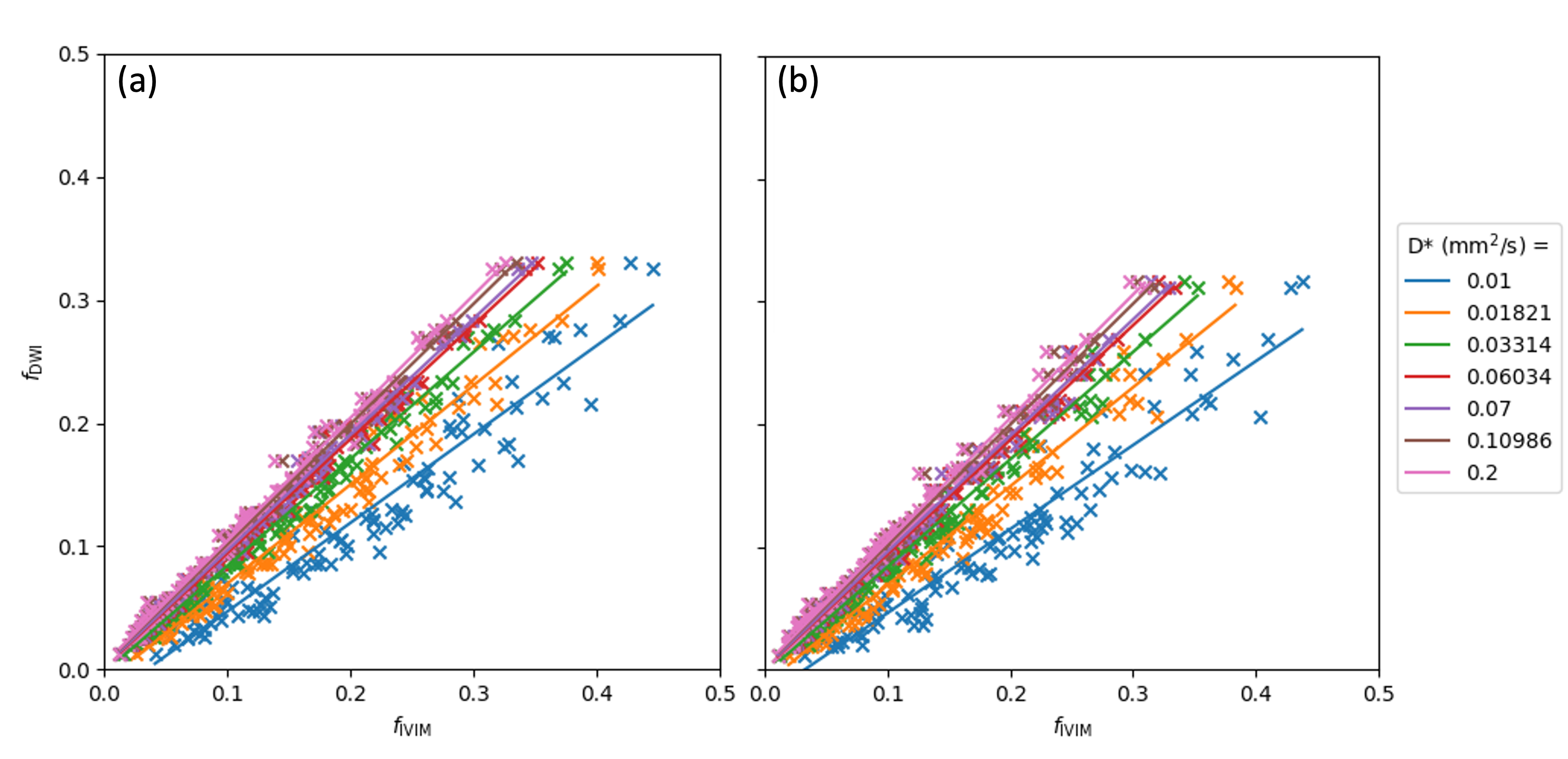
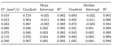
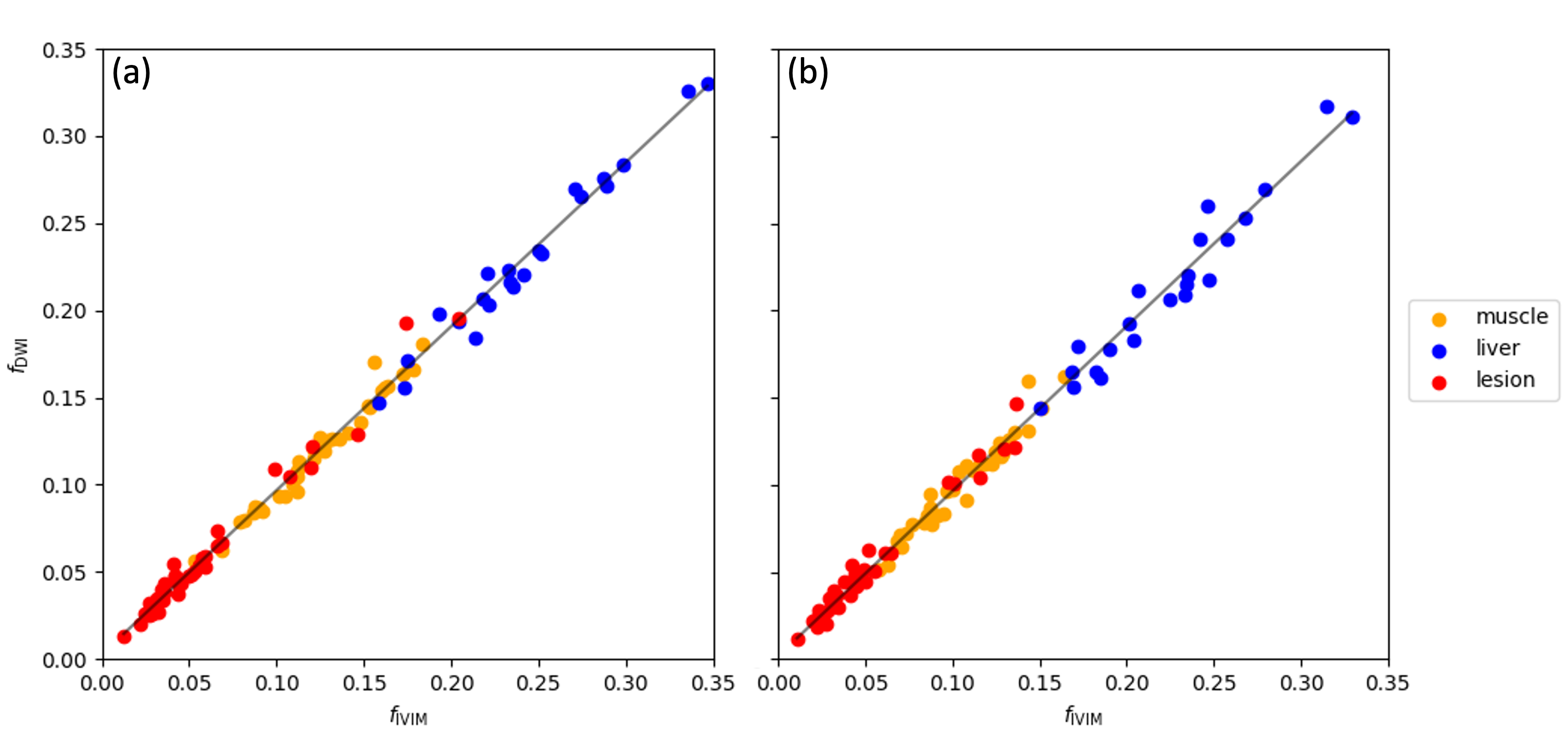
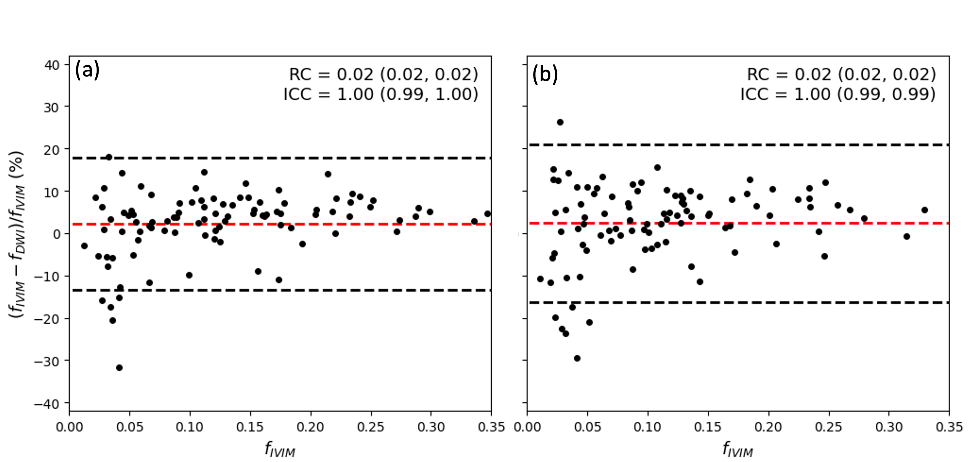
96 ROIs were analysed from 37 scans, with 37 ROIs drawn in disease and muscle, and 22 in liver. Figure 1 displays strong correlations (R2 > 0.7) between mean and median values of $$$f_{DWI}$$$ and $$$f_{IVIM}$$$ for all assumed D* values, and for larger D* values there is nearly a 1:1 relationship (Table 1).Tissue class separation was observed using both fitting methods (when assuming D*=70×10⁻³mm²/s), as illustrated Figure 2. Bland-Altman analysis (Figure 3) reveals $$$f_{DWI}$$$ underestimates $$$f_{IVIM}$$$ by a nominal amount (~2.3%).
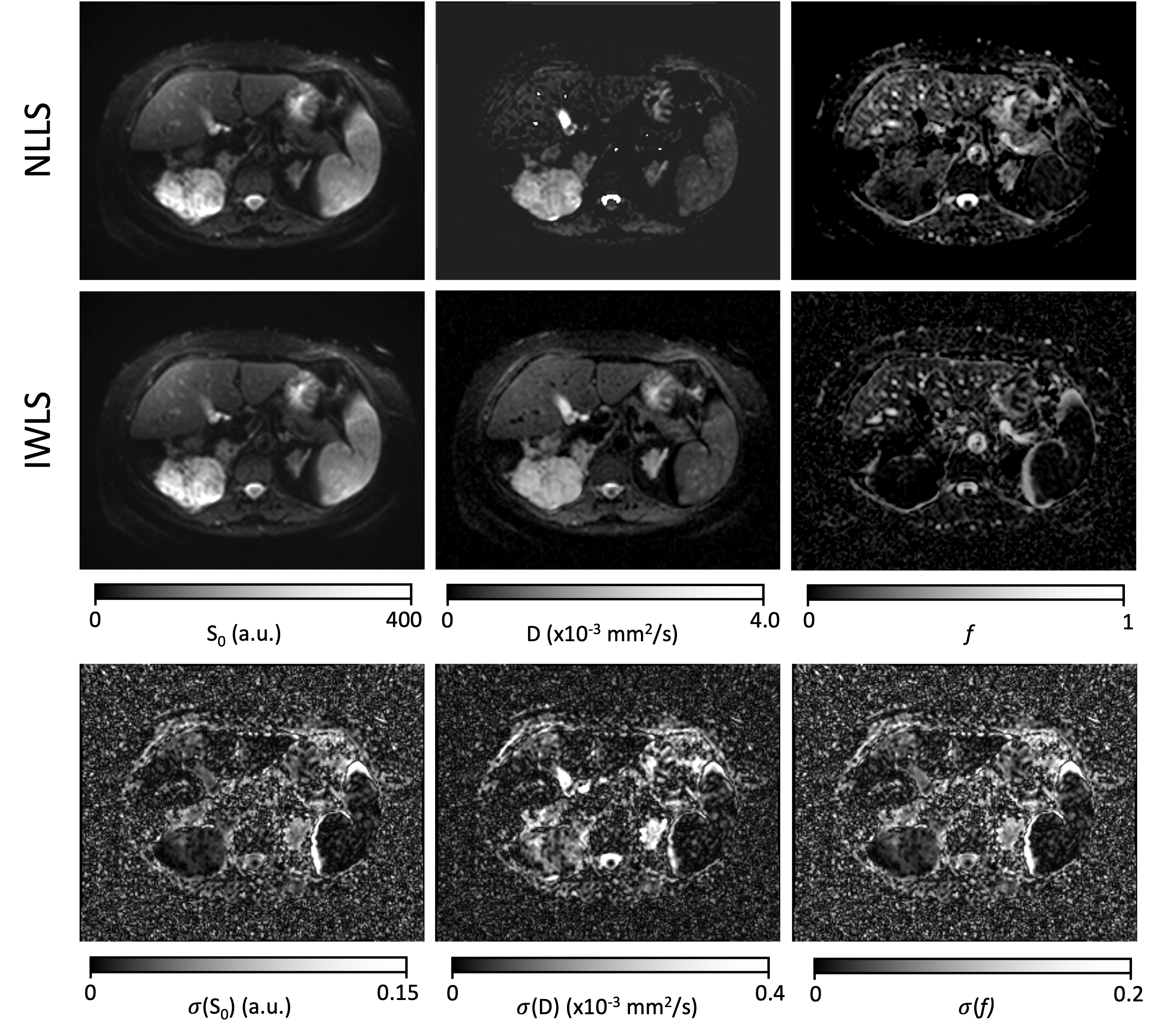
Figure 4 shows parameter maps fitted with both methods, along with uncertainty maps estimated using IWLS. Our approach resulted in significantly reduced fitting time compared to non-linear IVIM modelling with 8 b-values: 0.32 versus 249 seconds for a single slice on a personal machine.
Discussion
Strong correlation was achieved between mean and median values of $$$f_{DWI}$$$ and $$$f_{IVIM}$$$ though the former underestimated the true value by a small amount at our selected fixed D*. This likely results from the assumption that perfusion effects are only evident at b=0s/mm² in the linear model. Improvements might be seen by selecting a b-value of 100-150s/mm2 instead of 50s/mm2[7].Both $$$f_{DWI}$$$ and $$$f_{IVIM}$$$ distinguished between liver, muscle, and tumour, with liver having highest values followed by muscle then disease. This is consistent with expected values for liver and muscle[8,9]. However, lesion values were lower compared with other studies, possibly due to the difference in sarcoma subtypes[10].
The value of D* cannot be calculated from the linear model, however previous studies have shown D* from IVIM fitting has poorer repeatability than f[11]. Therefore, f could potentially be derived with acceptable repeatability for clinical applications.
Conclusion
The proposed model offers two key advantages: its linear nature enables faster fitting alongside parameter uncertainty estimation with IWLS and it reduces the required b-values. Using this model, $$$f_{DWI}$$$ can be estimated with just 3 non-zero b-values from clinical DWI and one additional acquisition at b=0 s/mm². This might allow for wider adoption of IVIM fitting in cases with limited acquisition time, such as whole-body MRI protocols, while also providing clinicians with parameter uncertainty maps. Further prospective testing with clinical DWI is required to confirm the accuracy of the model and correct for bias in $$$f_{DWI}$$$.Acknowledgements
This study represents independent research funded by the National Institute for Health and Care Research (NIHR) Biomedical Research Centre at The Royal Marsden NHS Foundation Trust and The Institute of Cancer Research, London, and by the Royal Marsden Cancer Charity. The views expressed are those of the author(s) and not necessarily those of the NIHR or the Department of Health and Social Care.References
1. Koh DM, Collins DJ, Orton MR (2011) Intravoxel incoherent motion in body diffusion-weighted MRI: Reality and challenges. Am J Roentgenol 196:1351–1361.
2. Winfield JM, Miah AB, Strauss D, et al (2019) Utility of multi-parametric quantitative magnetic resonance imaging for characterization and radiotherapy response assessment in soft-tissue sarcomas and correlation with histopathology. Front Oncol 9:446650.
3. Virtanen P, Gommers R, Oliphant TE, et al (2020) SciPy 1.0: fundamental algorithms for scientific computing in Python. Nat Methods 17:261–272.
4. Gurney-Champion OJ, Klaassen R, Froeling M, et al (2018) Comparison of six fit algorithms for the intra-voxel incoherent motion model of diffusion-weighted magnetic resonance imaging data of pancreatic cancer patients. PLoS One 13:e0194590.
5. Park HJ, Sung YS, Lee SS, et al (2017) Intra-voxel incoherent motion diffusion-weighted MRI of the abdomen: The effect of fitting algorithms on the accuracy and reliability of the parameters. J Magn Reson Imaging 45:1637–1647.
6. Blackledge MD, Tunariu N, Zugni F, et al (2020) Noise-Corrected, Exponentially Weighted, Diffusion-Weighted MRI (niceDWI) Improves Image Signal Uniformity in Whole-Body Imaging of Metastatic Prostate Cancer. Front Oncol 10:704.
7. Kooreman ES, van Houdt PJ, Keesman R, et al (2021) Daily Intravoxel Incoherent Motion (IVIM) In Prostate Cancer Patients During MR-Guided Radiotherapy—A Multicenter Study. Front Oncol 11:705964.
8. Zheng CJ, Xiao BH, Huang H, et al (2022) Bi-exponential fitting excluding b=0 data improves the scan-rescan stability of liver IVIM parameter measures and particularly so for the perfusion fraction. Quant Imaging Med Surg 12:3288–3299.
9. Englund EK, Reiter DA, Shahidi B, Sigmund EE (2022) Intravoxel Incoherent Motion Magnetic Resonance Imaging in Skeletal Muscle: Review and Future Directions. J Magn Reson Imaging 55:988–1012.
10. Zhang K, Dai Y, Liu Y, et al (2022) Soft tissue sarcoma: IVIM and DKI parameters correlate with Ki-67 labeling index on direct comparison of MRI and histopathological slices. Eur Radiol 32:5659–5668.
11. Andreou A, Koh DM, Collins DJ, et al (2013) Measurement reproducibility of perfusion fraction and pseudodiffusion coefficient derived by intravoxel incoherent motion diffusion-weighted MR imaging in normal liver and metastases. Eur Radiol 23:428–434.
Figures