2478
Automatic Segmentation and Quantitative Measurement of Deep Medullary Veins Diameter1School of Biomedical Engineering, ShanghaiTech University, Shanghai, China
Synopsis
Keywords: Software Tools, Quantitative Imaging
Motivation: Deep medullary veins (DMVs) stenosis may be one of the causes of small vessel disease, so non-invasive tool for its assessment is desired.
Goal(s): Developing automatic DMV segmentation and diameter quantification methods for assessing DMV stenosis.
Approach: We trained an automatic segmentation model and proposed a DMV diameter quantification method by analyzing the complex MRI signals at sub-voxel scale.
Results: The segmentation model achieved satisfactory performance. The accuracy of the diameter quantification method was verified in phantoms. The fitted DMV diameter distribution was close to earlier ex-vivo report and showed strong correlation with DMV susceptibility from quantitative susceptibility mapping.
Impact: Our approach can serve as a useful automatic pipeline to study the role of DMV stenosis in the pathogenesis of small vessel disease.
Introduction
Venous collagenosis (VC) may cause stenosis of deep medullary veins (DMVs), which might be a pathogenic factor of small cerebral vascular disease (CSVD).1-3 However, due to small diameters (100-250$$$\mu m$$$) of DMVs4 and time-consuming visual assessment5, narrowing of their calibers are difficult to detect in MRI images. Here, we proposed an automatic DMV diameter measurement method by training automatic DMV segmentation model and fitting the measured complex images surrounding the vein with physics based model images.Theory
If a long blood vessel is modeled as a cylinder and divided into n segments along the axis, the phase shifts caused by the magnetic field generated by the vessel inside the cylinder ($$$\phi_{in}$$$) and at point p outside the cylinder ($$$\phi_{out}$$$) are $$$\phi_{in} = {\gamma TEB}_{0}\Delta\chi\left( 3{cos}^{2}\theta_{vessel} - 1 \right)/6$$$ and $$$\phi_{out} = ~\gamma TE\mu_{0}/4\pi{\sum\limits_{i = 1}^{n}{m_{i}\left( 3{cos}^{2}\theta_{ip} - 1 \right){/r}_{ip}^{3}}}$$$ , respectively, where $$$\gamma$$$ is the gyromagnetic ratio, $$$TE$$$ the echo time, $$$B_{0}$$$ the main magnetic field, $$$\Delta\chi$$$ the blood-tissue susceptibility difference, $$$\mu_{0}$$$ the magnetic permeability, $$$m_{i}$$$ is the magnetic moment of the vessel segments which is defined as $$$m_{i} = ~{\pi B}_{0}\mathrm{\Delta}\chi a^{2}l_{i}/\mu_{0}$$$, where $$$a$$$ is the vessel radius. A detailed schematic diagram of the cylinder model is shown in Fig. 1. Combining the calculated phase value with the magnitude signal of the vessel and surrounding tissue, the complex images can be obtained at 3D sub-voxel scale. Convolving this complex images with point spread function (PSF)6 can account for partial volume effect (PVE). With $$$\Delta\chi$$$ and blood signal intensity as fixed parameters,, tissue signal intensity and the spatial position of the vessel axis approximated by a cylinder as free parameters, the complex image can be calculated and fitted to the measured images to obtain vessel diameters.Methods
First, we performed phantom studies to verify our method. A total of 8 graphite rods with different diameters (0.32 – 0.70 mm) were uniformly placed in a cylindrical container filled with water (Fig. 3A). The GRE images of the phantom were obtained on a 3T MR scanner (uMR890, United Image Healthcare) with the following parameters: TR = 28.6ms; TE = 3.7, 6.9, 10, 13, 17, 20, 23ms; resolution = 0.72×0.72×0.72 mm3. For in vivo study, 20 healthy volunteers with written informed consents were scanned on a 7T Siemens Magneton MRI scanner using a GRE sequence (TR = 21ms; TE1/TE2 = 7.59/15ms; resolution = 0.43×0.43×0.4 mm3).A 3D-UNet model provided by nnU-Net framework7 was trained to segment DMVs using both magnitude and phase images as input and manually drawn masks as ground truth. 19 subjects were used for training and remaining 1 subject for testing prediction accuracy using Dice similarity coefficient (DSC), positive predictive value (PPV), and sensitivity (SEN).
DMV and graphite rod diameters were calculated using our method for each DMV vessel cluster obtained from 3D-UNet segmentation and manually labeled graphite masks, respectively. In addition, the calculated DMV diameter was compared with its mean susceptibility generated by the STAR-QSM8 algorithm.
Results and Discussion
The output of DMV segmentation model is shown as an overlay in Fig. 2A in a representative slice. The average DSC, PPV and SEN achieved on every subject are all greater than 0.7 as shown in Fig. 2B. The top and bottom rows of Fig. 3B show the measured and fitted phase map, respectively, surrounding graphite rods with different diameters. There is a close match between the measured and true graphite rods diameters, assuming a $$$\Delta\chi$$$ of 100 ppm between water and graphite (linear regression R2 = 0.941 and slope = 0.963) as shown in Fig. 3C. Assuming a different value for $$$\Delta\chi$$$ will change the slope of the fitted line, but the proportionality relationship will not be affected.Fig. 4A shows the measured and fitted phase pattern in four continuous representative slices around a DMV. The DMV diameters obtained by fitting were distributed between 100$$$\mu m$$$ and 300$$$\mu m$$$ with a peak at ~160$$$\mu m$$$, as displayed in Fig. 4B, consistent with previous results. As shown in Fig. 4C, the mean QSM value of DMVs showed a strong correlation with the fitted diameter (p < 2.2 × 10⁻¹⁶, Spearman test), suggesting that the QSM results of DMV are strongly affected by partial volume effects.
Conclusion
Our study demonstrates that accurate segmentation of DMV can be achieved using a 3D-UNet model. Furthermore, DMV size can be quantitatively measured. The combined automatic segmentation and quantification tools may facilitate the study of the role of DMV stenosis in the pathogenesis of CSVD.Acknowledgements
The work was partly supported by NIH grant 5R21NS095027-02.References
1. Moody DM BW, Challa VR, Anderson RL. Periventricular venous collagenosis: association with leukoaraiosis. Radiology. 1995 Feb;194(2):469-76.
2. Wang JY, Li JY, Luo D, Huang MY, Ao DH, Liu Xn, et al. Extracellular Vesicles Play a Central Role in Cerebral Venous Disease‐Associated Brain Atrophy. Advanced Science. 2023;10(27).
3. Keith J, Gao FQ, Noor R, Kiss A, Balasubramaniam G, Au K, et al. Collagenosis of the Deep Medullary Veins: An Underrecognized Pathologic Correlate of White Matter Hyperintensities and Periventricular Infarction? Journal of neuropathology and experimental neurology. 2017;76(4):299-312.
4. Hooshmand I RA, Stein RL. Radiographic anatomy of normal cerebral deep medullary veins: criteria for distinguishing them from their abnormal counterparts. Neuroradiology. 1974:7(2):75-84.
5. Kuijf HJ, Bouvy WH, Zwanenburg JJM, Razoux Schultz TB, Viergever MA, Vincken KL, et al. Quantification of deep medullary veins at 7 T brain MRI. European Radiology. 2016;26(10):3412-8.
6. Zong X, Lin W. Quantitative phase contrast MRI of penetrating arteries in centrum semiovale at 7T. NeuroImage. 2019;195:463-74.
7. Isensee F, Jaeger PF, Kohl SAA, Petersen J, Maier-Hein KH. nnU-Net: a self-configuring method for deep learning-based biomedical image segmentation. Nat Methods. 2021;18(2):203-11.
8. Wei H, Dibb R, Zhou Y, Sun Y, Xu J, Wang N, et al. Streaking artifact reduction for quantitative susceptibility mapping of sources with large dynamic range. NMR Biomed. 2015;28(10):1294-303.
Figures
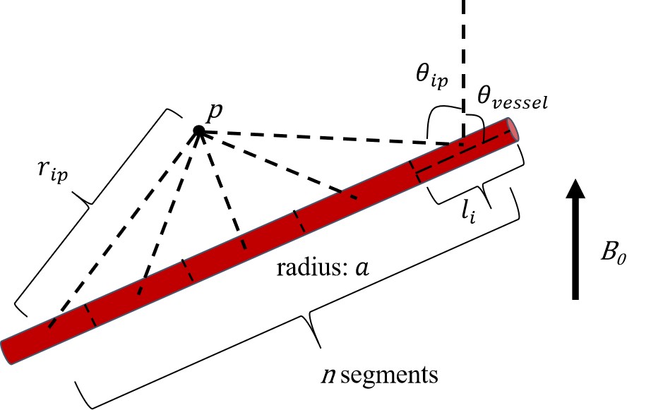
Figure 1: The diagram of the phase value calculation model. θvessel is the angle between vessel and B0, rip the length of the line from point p to the center of the vessel segment i and θip the angle between B0 and this line, li the length of vessel segment i, and a the vessel radius.
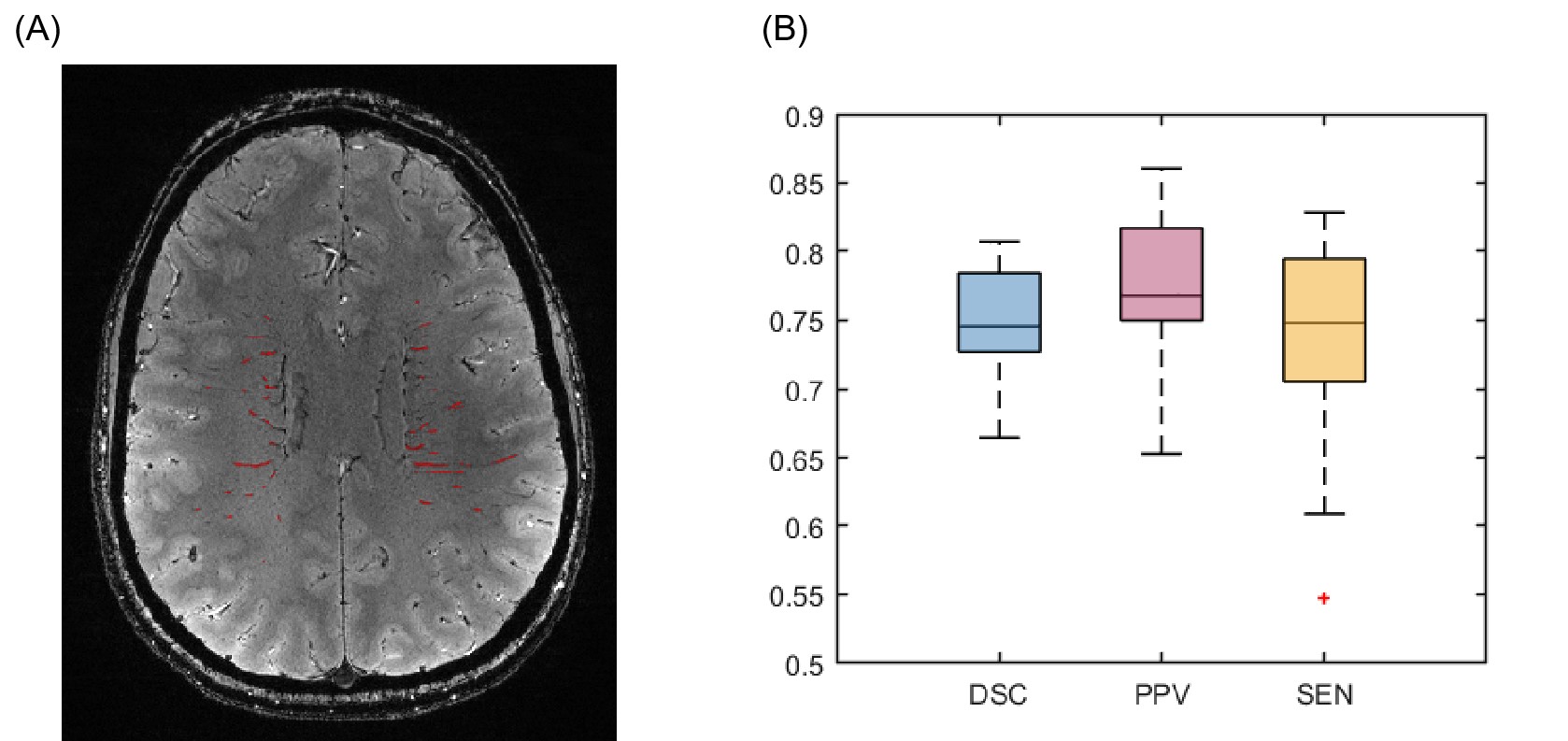
Figure 2: (A) The DMV mask (red voxels) delineated by the trained segmentation model overlaid on magnitude image. (B) Boxplot of DSC, SEN and PPV from all 20 trained segmentation models.
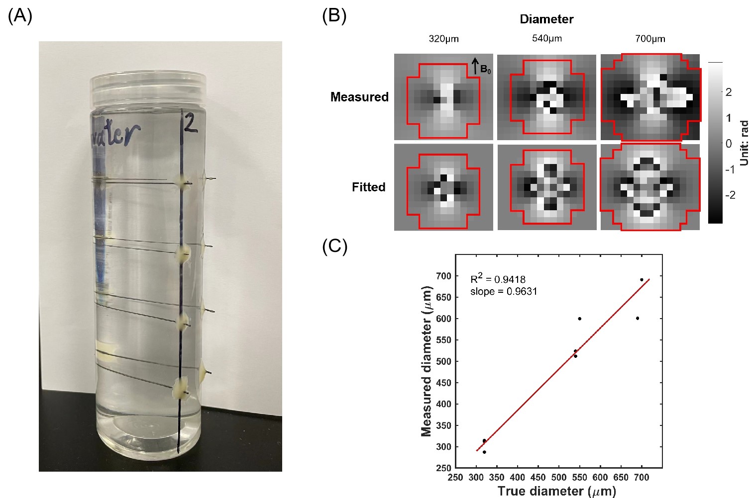
Figure 3: (A) A picture of the graphite phantom. (B) Top row: the phase pattern produced by graphite rods with diameters of 320μm, 540μm,and 700μm, respectively. Bottom row: the corresponding phase maps calculated from the fitted complex images. Only the voxels within the red contour were used for the fitting. (C) Scatter plot of measured versus true diameters of graphite phantoms. The red line shows the linear regression (y=kx) to the data.
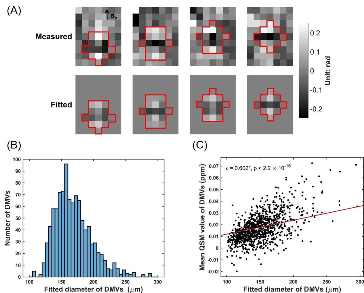
Figure 4: (A) Top row: measured phase maps around a DMV in four continuous slices. Bottom row: the corresponding fitted phase maps calculated from the fitted complex image. Only voxels within the red contours were used for the fitting. (B) The distribution of the fitted DMV diameters. (C)The scatter plot of the mean susceptibility values of DMVs vs. the corresponding fitted diameters.