2463
Investigation and validation for cortical laminar structures of myelin and iron using χ-separation (chi-separation)1Department of Electrical Computer Engineering, Seoul National University, Seoul, Korea, Republic of, 2Department of Radiology and Radiological Science, Johns Hopkins University School of Medicine, Baltimore, MD, United States, 3F.M. Kirby Research Center for Functional Brain Imaging, Kennedy Krieger Research Institute, Baltimore, MD, United States
Synopsis
Keywords: Susceptibility/QSM, Susceptibility, Gray Matter/ Ex-Vivo Applications
Motivation: Previous studies have demonstrated the correlations between iron and paramagnetic susceptibility and myelin and diamagnetic susceptibility. However, there has yet to be a quantitative layer-wise comparison with histology.
Goal(s): Our objective is to validate laminar structures of χ-separation against histology in V1.
Approach: In V1, we performed laminar profiling of χ-separation, iron-, and myelin histology. The profile was obtained by sampling points at 5% intervals along the cortical depth, oriented perpendicularly to the cortex.
Results: The cortical depth profile reveals that both χpara with iron histology and χdia with myelin staining exhibit similar profiles and peaks at the location of the Gennari line.
Impact: By comparing the cortical depth profile in the V1 region including the location of the Gennari line between χ-separation and histology, we have confirmed that χ-separation (χpara, χdia) accurately represents the quantitative amounts of iron and myelin with precision.
Introduction
χ-separation (chi-separation) can separate paramagnetic and diamagnetic susceptibilities1. Previous studies have confirmed the relationship between iron and paramagnetic susceptibility, and myelin and diamagnetic susceptibility1–4, respectively, but quantitative layer-wise comparison with ex-vivo histology is yet to be done.Primary visual cortex (V1) can be distinguished by the presence of the Gennari line located in a sublayer internal granular layer (IVb)4-5. The Gennari line in V1 exhibits a line-shaped distribution where both iron and myelin distributions are more prominent than the surrounding layers. Therefore, these distinctive structures can serve as valuable references to evaluate the relationship between χ-separation maps and iron and myelin accumulations.
Therefore, this study aims to quantitatively assess how precisely χ-separation can distinguish susceptibility sources by comparing layer-wise profiles in iron-, and myelin-histology and ex-vivo χ-separation maps in the V1 region.
Methods
An ex-vivo human brain specimen, containing V1, was scanned1 at 7T MRI (Siemens Terra, Erlangen, Germany). 3D multi-echo gradient-echo were used with the following parameters: FOV = 77 × 77 × 64 mm3, voxel size = 0.3 × 0.3 × 0.5 mm3, TR = 300 ms, TE = 3.9:6.5:36.4 ms. For 3D multi-echo spin-echo, the parameters had the same FOV and resolution as the gradient-echo acquisition, TR = 50 ms, TE=14:14:70 ms. χ-separation is conducted using local field6,7, R2*8, and R29 maps which are processed from acquired data. After the MRI scan, the specimen was utilized for LFB myelin staining and LA-ICP-MS for iron1. LFB myelin staining image representing optical density, which has low intensity in myelinated areas, is transformed into an absorbance map using the Beer-Bouguer-Lambert law10.$$log(I_0/I)=A$$
V1 ROI is manually segmented using AutoCAD (version 2024, Autodesk Inc.) considering microstructural and macroscopic features5in χ-separation and histology maps (Figure 1a). Cortex boundaries were defined as follows: Interface between CSF and cortex was defined as an outer contour with 0% depth. The border between the deepest cortical sublayer VI and the white matter5 was defined as an inner contour with 100% depth (Figure 1b). Depth trajectory is defined as a line perpendicular to cortical layers, heading to the white matter. Evenly spaced trajectories are manually drawn along the cortex, without intersection with neighboring trajectories11 (Figure 1c). Within the ROIs, there exist 54 depth trajectories.
Additionally, cortical depth-wise points were sampled over each depth trajectory, dividing the trajectory into 20 segments along the cortical depth with 5% increments. (Figures 1d and 2) Using depth-wise samples, laminar profiles were acquired by averaging intensity at each depth. Cortical laminar profiles were z-score normalized for quantitative comparison. This normalization enabled a quantitative assessment of intermodal differences in tendencies of the cortical profile, including the peak of the Gennari line. Laminar profiles between χpara and iron histology; and χdia and myelin staining were visually assessed and similarity was measured using the mean Euclidean Distance (ED)5.
Results
Figure 2 depicts the segmented cortical layers in each χ-separation and histology. The resulting segments agree well with each other.In Figure 3, laminar profiles of χdia and myelin staining are plotted. Both profiles display increasing values as they get deeper and peak at 65% depth. The profile values decrease until 75 to 80% depth and continue to rise until 100% depth. These features are similar to the previously reported depth of the Gennari line and the shape of the laminar profile5. When z-score normalized profiles are compared, they exhibit similarity, with a mean Euclidean Distance of 0.909±0.143.
Figure 4 illustrates the laminar profiles of χpara and iron histology. Both profiles display increasing values with depth, peaking at 65% depth, coinciding with the previously reported depth of the Gennari line5, then decreasing until 100% depth. The z-score normalized profiles demonstrate a notable similarity, with a mean Euclidean distance of 0.357±0.043.
Conclusion and Discussion
In this study, we investigated the laminar profiles of the primary visual cortex within χ-separation maps and histology maps. When manually segmented laminar profiles are compared, the results show that the profiles of iron histology and χpara, and myelin histology and χdia coincide throughout the cortex, respectively, including a peak at the Gennari line.Although we performed manual segmentation to maximize the alignment of segmented cortical boundaries, the boundaries were less distinct in the iron histology, resulting in potential inconsistencies. These issues might be addressed through a comparative analysis of the maps after registration or by employing alternative segmentation criteria.
The results presented in this work are in line with the previous observations and reinforce the connection between chi-separation results and histology. Based on these results, layer-wise analysis of other cortex regions using χ-separation could be possible.
Acknowledgements
This work was supported by the Brain Korea 21 Plus Project in 2023.
This work has been supported by the National Research Foundation of Korea (NRF) grant funded by the Korea government (MSIT) (NRF-2021R1A2B5B03002783).
This work is supported by Institute of New Media and Communications (INMC), SNU
References
1. Shin, H.-G. et al. χ-separation: Magnetic susceptibility source separation toward iron and myelin mapping in the brain. NeuroImage 240, 118371 (2021).
2. Kim, W. et al. χ-Separation Imaging for Diagnosis of Multiple Sclerosis versus Neuromyelitis Optica Spectrum Disorder. Radiology 307, e220941 (2023).
3. Lee, S., Shin, H.-G., Kim, M. & Lee, J. Depth-wise profiles of iron and myelin in the cortex and white matter using χ-separation: A preliminary study. NeuroImage 273, 120058 (2023).
4. Fukunaga, M. et al. Layer-specific variation of iron content in cerebral cortex as a source of MRI contrast. Proc. Natl. Acad. Sci. 107, 3834–3839 (2010).
5. Eickhoff, S. et al. High‐resolution MRI reflects myeloarchitecture and cytoarchitecture of human cerebral cortex. Hum. Brain Mapp. 24, 206–215 (2005).
6. Dymerska, B. et al. Phase unwrapping with a rapid opensource minimum spanning tree algorithm (ROMEO). Magn. Reson. Med. 85, 2294–2308 (2021).
7. Wu, B., Li, W., Guidon, A. & Liu, C. Whole brain susceptibility mapping using compressed sensing. Magn. Reson. Med. 67, 137–147 (2012).
8. McGibney, G., and M. R. Smith. “An unbiased signal‐to‐noise ratio measure for magnetic resonance images.” Medical physics 20.4 (1993): 1077-1078.
9. McPhee, K. C. & Wilman, A. H. T2 quantification from only proton density and T2-weighted MRI by modelling actual refocusing angles.pdf. NeuroImage 118, 642–650 (2015).
10. Bouguer, Pierre (1729). Essai d’optique sur la gradation de la lumière [Optics essay on the attenuation of light] (in French). Paris, France: Claude Jombert. pp. 16–22.
11. Schleicher, A. et al. A stereological approach to human cortical architecture: identification and delineation of cortical areas. J. Chem. Neuroanat. 20, 31–47 (2000).
Figures
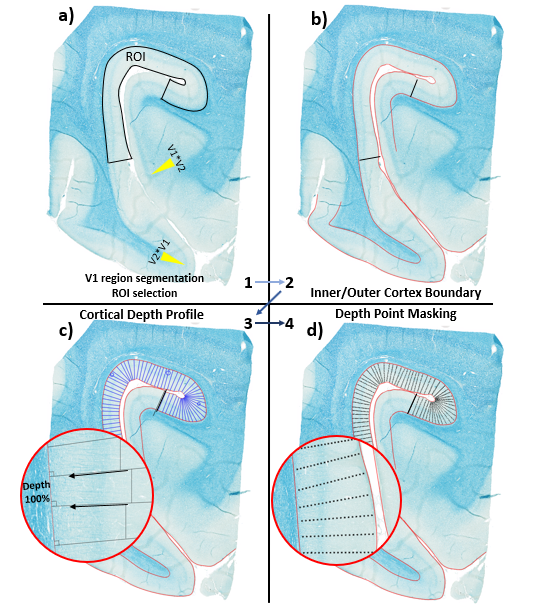
Fig. 1. Process of manual segmentation. Myelin staining was used to illustrate this process because the image contrast clearly showed the manual segmentation lines. a) V1 region is found in myelin stained image. b) The inner and outer cortex boundaries were manually segmented with reference to image contrast. c) Cortical depth profiles were drawn perpendicular to the cortex boundary created in b) and were evenly spaced. d) ninety equidistant points along the cortical depth profile lines were chosen as depth points, which were used to mask pixels.
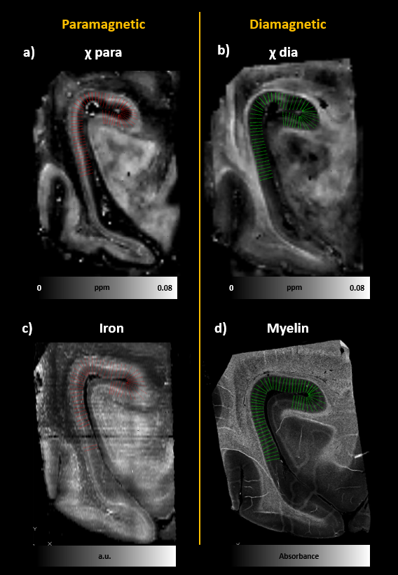
Fig. 2. Segmented layers in χ-separation maps and histology. a) and b) The inner cortical boundary for χ-separation was extracted from χdia, where the inner cortical boundary was distinctly visible. The outer cortical boundary was obtained from χpara, where the outer cortical boundary was clearly visible. χdia and χpara share the same depth-wise pixel mask. c) For iron, there is area where four depth trajectories are not drawn due to an artifact in the middle. d) LFB myelin staining, with image contrast opposite to other modalities, was converted using the Beer-Bouguer-Lambert law.
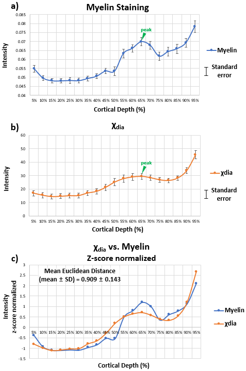
Fig. 3. Comparison of laminar profiles of χdia and myelin histology. a) The laminar profile of myelin histology shows an intensity peak at 65% depth. b) The laminar profile of χdia also has a Gennari line peak at 65%. c) Both z-score normalized laminar profiles of myelin and χdia display increasing values as getting deeper and decrease until 75 to 80% depth and continue to rise until 100% depth. The mean Euclidean distance is 0.909 ± 0.143.
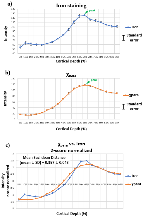
Fig. 4. Comparison of laminar profile of χdia and myelin histology. a) The laminar profile of iron histology shows an intensity peak at 65% depth. Standard error is relatively lower than in χpara vs. iron. b) The laminar profile of χpara also has a Gennari line peak at 65%. c) Both z-score normalized laminar profiles of χpara and iron display increasing values as getting deeper until 65% depth and decrease until 100% depth. The χpara vs. iron has a lower mean Euclidean Distance than the χdia vs. myelin, which means the laminar profiles of χpara vs. iron are more similar.