Introduction

The diffusivity of water increases with temperature. This affects the magnitude of signals measured in postmortem diffusion MRI¹. Optimally, the sample would be kept at a constant room temperature by cooling, but this is not always an option for large samples or demanding sequences. Large tissue samples eventually reach steady-state temperature after several hours of active scanning, but delaying data acquisition is not efficient and not always possible. We present a post-processing method to correct data acquired during temperature adaptation.

Methods

We assume that the sample temperature has reached steady-state for a subset of our total diffusion measurements, typically the last $$$M$$$ directions (if the dataset is ordered and the scan wasn't interrupted). We denote the set of b-values and gradient directions as $$$\{b_i,g_i\}$$$ and the steady-state subset as $$$\{b_i^{\prime},g_i^{\prime}\}$$$. We fit a DTI model² using only $$$\{b_i^{\prime},g_i^{\prime}\}$$$ and we predict a signal for each gradient direction in $$$\{b_i,g_i\}$$$ (for each voxel ($$$xyz$$$)). The predicted signal is $$$S_{i\text{,pred}}(xyz)=S_0\exp(-b_i(g_i^T{\cdot}D_{\text{fit}}(xyz){\cdot}g_i))=S_0\exp(-b_i\text{ADC}_i(xyz))$$$ where $$$\text{ADC}_i(xyz)$$$ is our estimate of the apparent diffusivity for the i-th gradient direction at steady state temperature for voxel (xyz). We model the effect of temperature as a multiplicative factor over the ADC; $$$\text{ADC}_{i\text{,obs}}=\alpha_i\cdot\text{ADC}_i$$$ where $$$\alpha_i$$$ depends on the temperature difference and is assumed to be constant over the whole volume. We first estimate $$$\alpha_i(xyz)$$$ voxel-wise for each volume by comparing the DTI prediction and the measured signal $$$S_{i\text{,obs}}(xyz)=S_0\cdot\exp(-b_i\cdot\alpha_i(xyz)\cdot\text{ADC}_i(xyz))$$$.
$$\frac{S_{i\text{,pred}}(xyz)}{S_{i\text{,obs}}(xyz)}=\frac{S_0\exp(-b_i\cdot\text{ADC}_i(xyz))}{S_0\exp(-b_i\cdot\text{ADC}_{i\text{,obs}}(xyz))}=\frac{\exp(-b_i\cdot\text{ADC}_i(xyz))}{\exp(-b_i\cdot(\alpha_i(xyz)\cdot\text{ADC}_i(xyz)))}$$
$$\Rightarrow\ln\frac{S_{i\text{,pred}}(xyz)}{S_{i\text{,obs}}(xyz)}=-b_i{\cdot}(1-\alpha_i(xyz))\cdot\text{ADC}_i(xyz)$$
$$\Rightarrow\alpha_i(xyz)=1+\frac{\text{ln}\frac{S_{i\text{,pred}}(xyz)}{S_{i\text{,obs}}(xyz)}}{b_i\cdot\text{ADC}_i(xyz)}$$
The voxel-wise estimation of $$$\alpha_i(xyz)$$$ is very noisy and biased by the tensor model. We therefore take the median over a brain mask for each volume; $$$\alpha_i=\text{median}_{\forall(xyz)\in\text{mask}}(\alpha_i(xyz))$$$. This last step enforces a constant temperature estimation for each volume. Lastly, we correct the signal at each volume by modulating the log-signal.
$$S_{i\text{,corr}}(xyz)=S_0\cdot\exp\left(\frac{1}{\alpha_i}\cdot\ln\frac{S_{i\text{,obs}}(xyz)}{S_0}\right)$$

Results

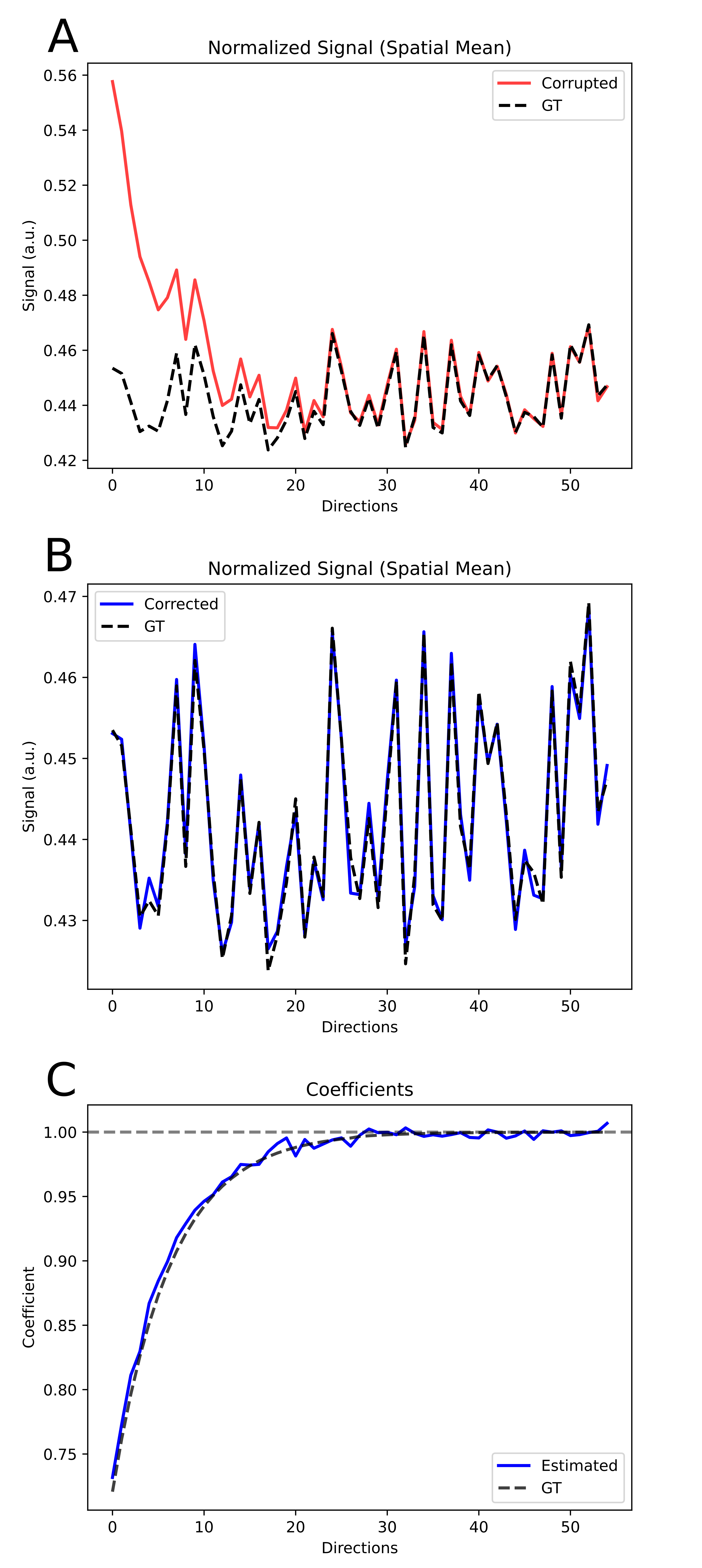
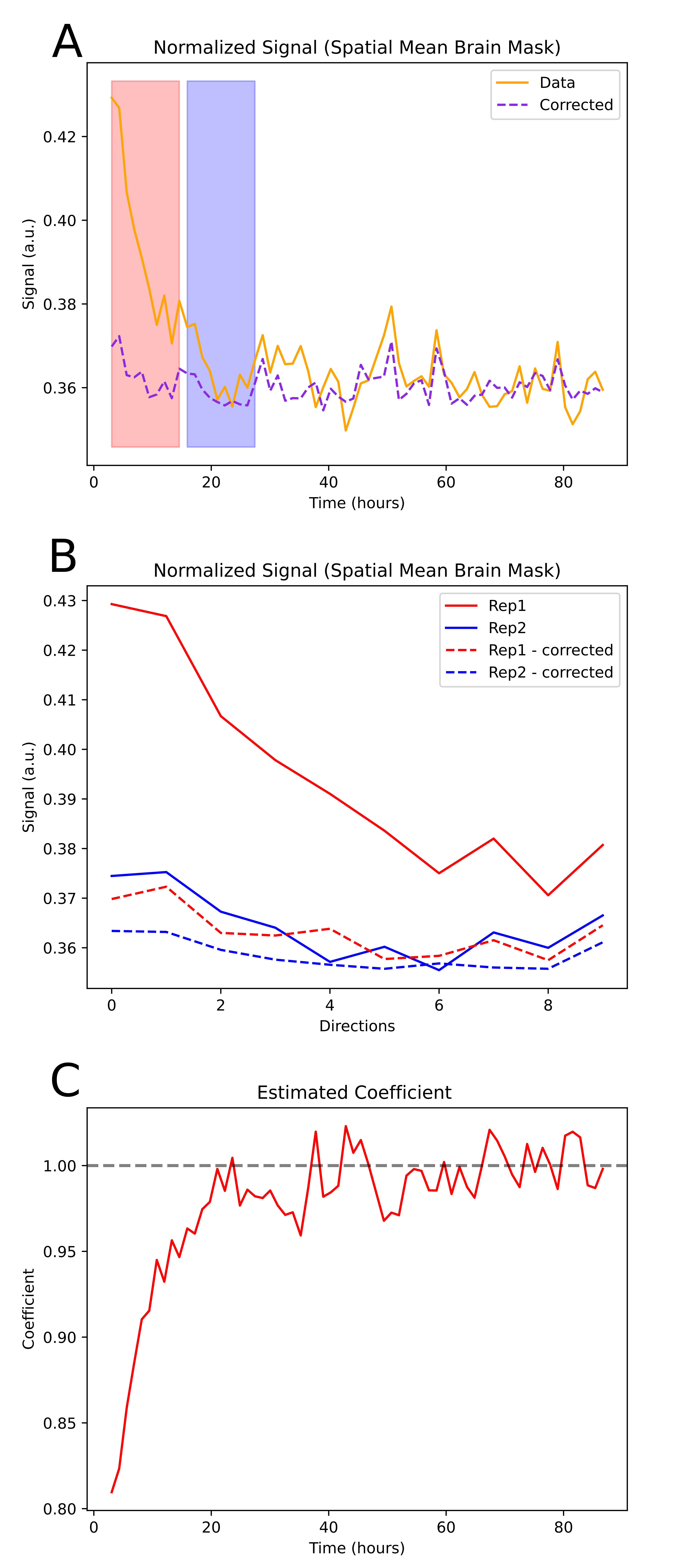
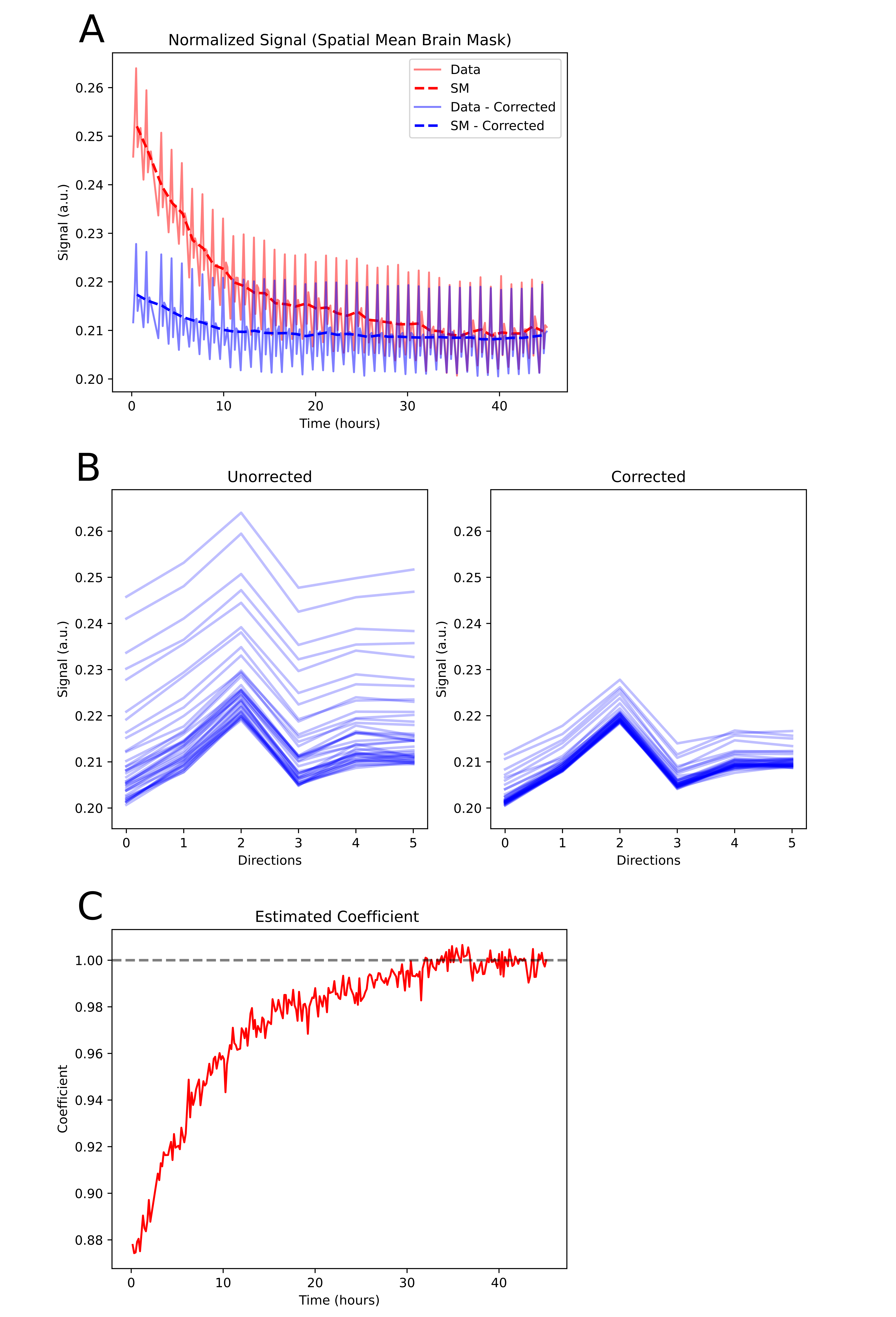
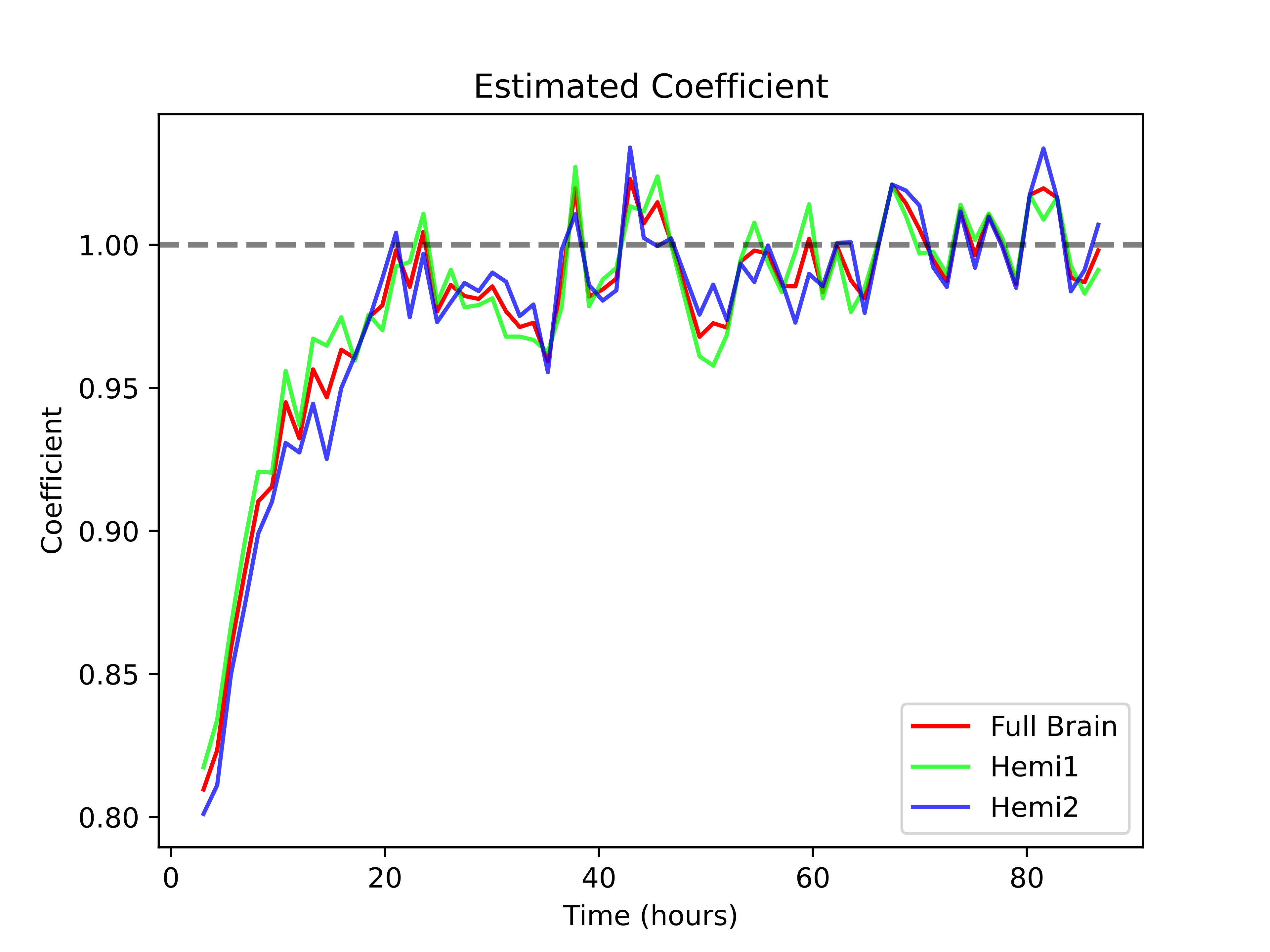
We first validate the method on synthetic data, generated by convolving crossing geometry fiber ODFs with diffusion kernels. We generated 1000 fODF and kernel pairs ($$$[75,90]$$$ degrees crossing angle, kernel $$$\text{MD}\in\left[\frac{0.6}{5},\frac{1.2}{5}\right]\,\frac{mm^2}{s}$$$) and computed a diffusion signal for $$$N=55$$$ directions at $$$b=5000\,\frac{s}{mm^2}$$$. We generated an exponential temperature coefficient curve (Fig.1C) designed to mimic a large total temperature increase of about $$$20^{\circ}\text{C}$$$ ³. We generated a second diffusion signal where the diffusivities were corrupted by these coefficients. We added Gaussian noise to both signals so that $$$\text{SNR}=50$$$. Fig.1A shows these two signals averaged over all fODFs. The temperature induced diffusivity drift is evident in the curves. Using the proposed method, we obtain a good estimation of the coefficients (Fig.1C) and we computed the corrected signal (Fig.1B), which almost perfectly matches the ground truth. For further illustration, we computed a spherical deconvolution⁴ on the signal with a tensor kernel of ratio 2. The angular error between the ground truth peaks and the deconvolution peaks were 8.36 degrees for the baseline, 10.35 degrees for the temperature corrupted, and 8.66 degrees for the corrected signal. We also compute the ratio of voxels with exactly 2 peaks and an angular error below 5 degrees (STAR, Success-To-Attempt Ratio). The STAR were $$$49.9\%$$$ for the baseline, $$$34.7\%$$$ for the corrupted and $$$48.3\%$$$ for the corrected signal. We qualitatively demonstrate the impact of the proposed method on two postmortem segmented EPI acquisitions⁵ on a preclinical Bruker Biospec 94/30 MRI system. Fig.2A shows the signal for a high resolution scan with $$$N=65$$$ directions. The acquisition included a 12h48m dummy scan of 10 diffusion directions at the beginning, followed by a repetition of the same directions. We corrected the data using the last 28 volumes for the tensor fit. The corrected signal shows less exponential decay (Fig.2A) and the agreement between the signal of the dummy directions and the repetition is greatly increased (Fig.2B). Fig.3A shows the signal for a low resolution scan with 40 repetitions of 6 directions. We apply the proposed method by fitting DTI to the last 23 repetitions. The corrected data show a much better agreement between the repetitions (Fig.3B). In Fig.4, we split the data from (Fig.3) by hemisphere and compute the volume-wise correction factor independently. The resulting curves demonstrate the stability of the coefficient estimation method.

Conclusion

We have demonstrated a simple, data-driven method to account for changing temperature during postmortem diffusion MRI acquisition without relying on a temperature probe and heat transfer models. This method may help to reduce the required dummy scans prior to reaching steady-state temperature. Future work will address the key assumption of uniform temperature within the sample.

Acknowledgements

This work was funded by the presidential funds of the Max Planck Society to the Inter-Institutional Research Initiative ‘Evolution of Brain Connectivity’.