Introduction

Magnetization-prepared (MP) GRE sequences improve the imaging speed in 3D T1ρ parameter mapping. However, this type of acquisition suffers from T1 recovery contamination and loss of MP contrast. 3D magnetization-prepared angle-modulated partitioned k-space spoiled gradient echo snapshots (MAPSS) sequence overcomes these limitations by repeating magnetization preparation with opposite phase cycling (PC) during MP and performing subtraction after reconstruction [1]. However, this approach doubles scan time and is prone to motion artifacts. Undersampling data acquisitions for different PC can compensate for long scan time. In addition, since MAPSS involves dynamic imaging, one can take advantage of spin lock time (TSL) dimension to further reduce scan time. In this work we propose three different undersampling strategies to reduce scan time and use deep learning to reconstruct images and evaluate performance of each strategy.

Methods

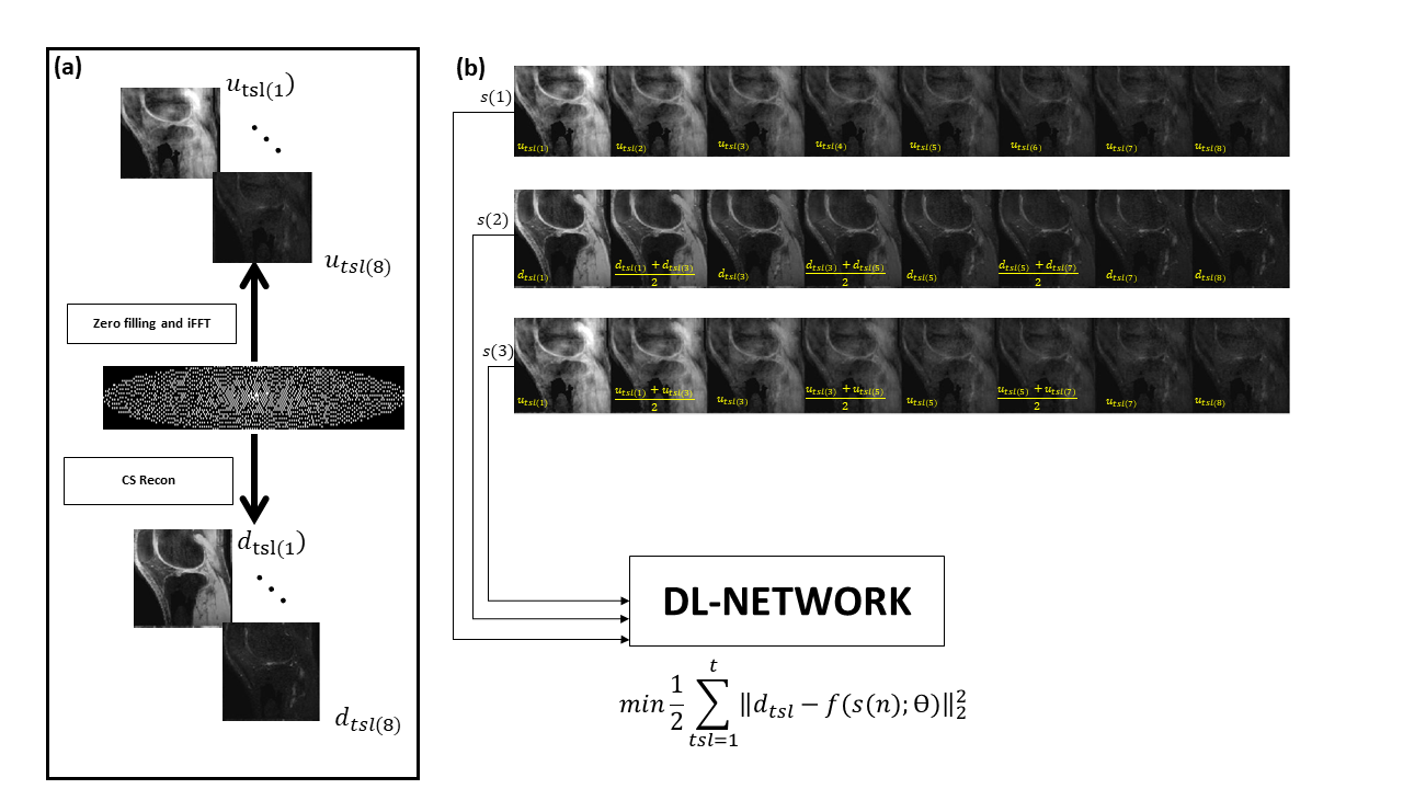
3D MAPSS sequences was acquired in sagittal plane in thirteen healthy volunteers on 3.0T Philips scanners with 1Tx/16Rx knee coil. Scan parameters inlcuded: FOV = 140×140×140 mm3, acquisition voxel size = 0.45×0.72×4 mm3 reconstructed to 512×512×30 matrix size, TR/TE = 7.3/3.7 ms, and bandwidth = 64.4 kHz, acceleration factor=4. Each acquisition with positive or negative PC [TSL=±0, ±10, ±20, ±30, ±40, ±50, ±60, and ±70ms] took 35.7s, leading to a total scan duration of 9 min 32 s for 16 acquisitions [2].

DL Reference:The vendor-specific wavelet-based compressed-SENSE reconstruction algorithm on the scanner was used to generate the complex 3D images per TSL. Next, each ±PC 3D dataset pair was subtracted to generate a single of 3D datasets free of T1 relaxation contaminations, leading to 8 independent datasets ($$$d_{tsl}$$$) with different TSLs from 16 acquisitions as reference (Figure 1, (a)).

Input: Coil combined k-space data from reference images were retrospectively undersampled with the same undersampling (acceleration factor=4) mask during acquisition followed by zero filling and iFFT to form images ($$$u_{tsl}$$$) with artifacts (Figure 1, (a)). Three different inputs were implemented one at a time for training (Figure 1, (b)):

$$$s(1)$$$: undersampled images ($$$u_{tsl}$$$) were input to the network for all 8 TSLs.
$$$s(2)$$$: Reference images ($$$d_{tsl}$$$) were input to the network while skipping every other dynamic (TSL=2,4,6) by replacing it with average of previous and next dynamic ($$$d_{tsl}(n) =(d_{tsl}(n-1) +d_{tsl}(n+1))/2 $$$)
$$$s(3)$$$: A combination of $$$s(1)$$$ and $$$s(2)$$$ strategies was used where only undersampled images ($$$u_{tsl}$$$) were used as input and every other dynamic was replaced with average of previous and next dynamic ($$${u_{tsl}}(n) =({u_{tsl}}(n-1) +{u_{tsl}}(n+1))/2 $$$).

Deep Learning: Fully convolutional neural network with contracting and expanding paths was designed. The contracting path included 6 blocks each consisting of convolution (3×3), activation function (ReLu), batch normalization and max pooling (3×3) [3]. Dynamics TSL=1:t) were added as additional channels. Each slice data were normalized along TSL direction. The following cost function was minimized during training:
$$min\frac{\text1}{\text2}\sum_{tsl=1}^t || d_{tsl}-f(s(n));\ominus||_2^2 $$
where $$$s(n)$$$ is the input of to the network and n represents each undersampling method. Θ corresponds to network weights for mapping ($$$f$$$).
Network parameters included Adam optimizer, learning rate 10-3, batch size=4, epochs=500. Training was performed on NVIDIA Tesla V100-SXM2-32GB with ~0.9 minutes per epoch.

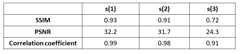
To compare the reference with the network output, correlation coefficient, peak signal-to-noise ratio (PSNR) and structural similarity index (SSIM) are reported. Qualitative impressions are provided.

Results

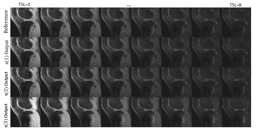
In Figure 2 comparison between reference (top), and network output for three undersampling strategies across TSLs shows both image quality and sharpness improvement compared with input images obtained from iFFT (Figure 1, (b)).$$$s(1)$$$ and $$$s(2)$$$ show comparable results to reference images including contrast and details. In $$$s(3)$$$ while input undersampling artifacts (Figure 1) have been successfully removed, contrast tend to be higher and some details have not been recovered. While later dynamics tend to be noisier on reference images, all three undersampling strategies show improved noise performance.

In Table 1. Comparison of SSIM, PSNR, and correlation coefficient shows, $$$s(1)$$$ has the best agreement with the reference images, followed by $$$s(2)$$$ with similar scores. $$$S(3)$$$ has the lowest agreement.

Discussion and Conclusion

While most undersampling strategies focus on designing undersampling masks, we explored inherent correlation in dynamic imaging with shared features to guide the network to further decrease scan time by excluding dynamic images during training. A combination of both k-space undersampling and skipping dynamics would allow to further shorten scan time by a large factor. Results can be further improved by adding signal model since there is an exponential decay across dynamics. In addition, including more training cases would increase network robustness. Motion was observed in a few subjects between datasets at different dynamics. Therefore, pre-training motion correction will further improve the network performance

Acknowledgements

No acknowledgement found.