2266
Fully Automated Whole-Leg multiparametric quantitative MRI processing, segmentation and analysis.1Department of Radiology, UMC Utrecht, Utrecht, Netherlands, 2Department of Neurology, BG-University Hospital Bergmannsheil gGmbH, Bochum, Germany
Synopsis
Keywords: Muscle, Quantitative Imaging, Analysis/Processing; Software Tools
Motivation: Quantitative magnetic resonance imaging (qMRI) is a common tool for assessing neuromuscular disorders, but its quantitative parameters often lack specificity and generally do not directly relate to muscle function.
Goal(s): In our ongoing MOTION study, we are collecting whole-leg qMRI data and assessing muscle structure, function, and lifestyle in a large cross-sectional cohort to identify confounding factors in qMRI evaluation.
Approach: To streamline data analysis for this cohort, we've developed a fully automated muscle-Bids-based data analysis pipeline, including automated muscle segmentation.
Results: Here, we introduce our data analysis pipeline, demonstrated using repeated scans of one volunteer.
Impact: The implementation of fully automated qMRI data processing streamlines large-scale studies and enhances its integration into clinical workflows. This standardization we expect to reduces variability for more dependable and reproducible outcomes.
Introduction
Magnetic resonance imaging (MRI) is widely used for assessing neuromuscular disorders(1). However, quantitative MRI (qMRI) parameters, while sensitive, often lack specificity and are not commonly associated with muscle function. In our ongoing MOTION study, we collect whole-leg qMRI data and evaluate muscle structure, function, and lifestyle in a large cross-sectional cohort to establish connections between qMRI and muscle function. To streamline data analysis for this cohort, we've developed a fully automated muscle-Bids-based data analysis pipeline, including automated muscle segmentation. Here, we introduce our openly available data analysis pipeline(2).Methods
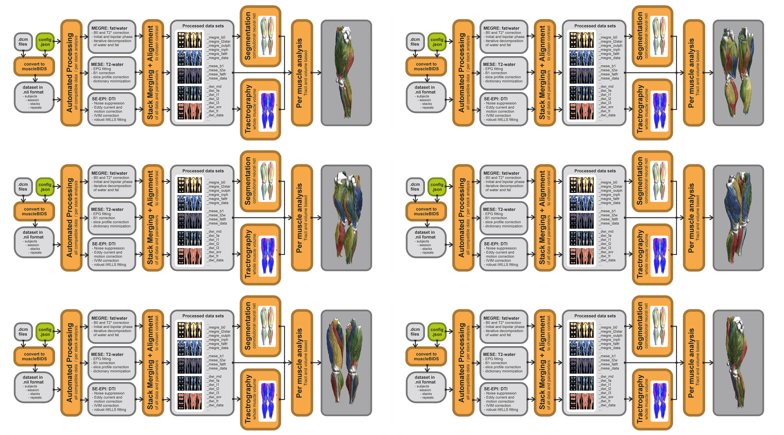
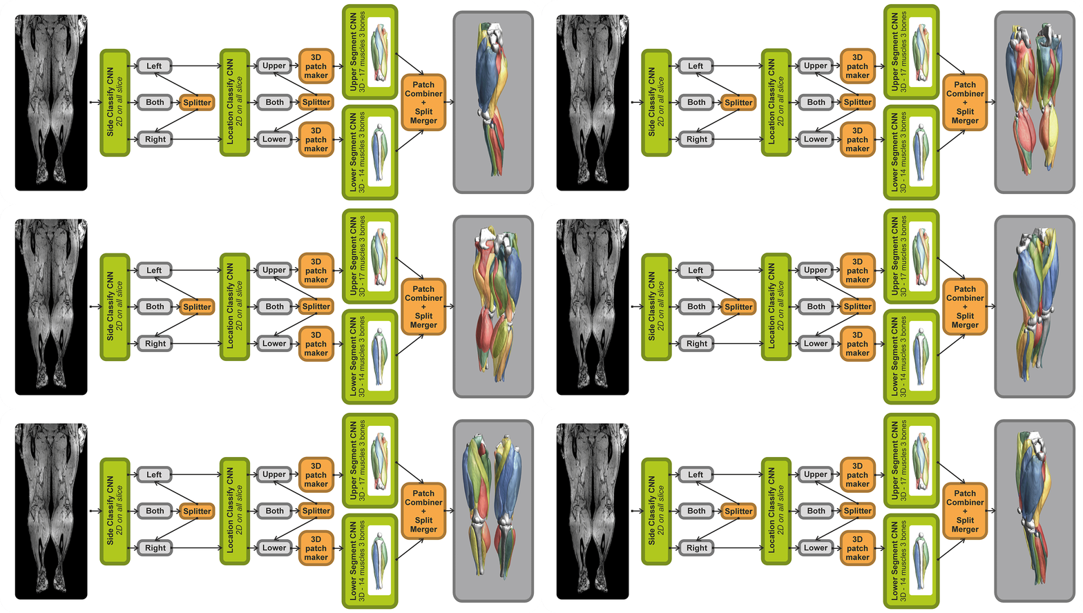
In this study, we obtained three full-leg qMRI datasets from a single male volunteer, covering from hip to ankle. The subject was scanned supine, with the ankle fixed in 20° plantar flexion using a footrest, while supporting the Popliteal Fossa and heel to prevent leg muscle compression. The MRI protocol (~45min) included 6 overlapping continuous stacks (30 mm) with a combined FOV of 480x276x966 mm³. This comprised ME-GRE (52s/stack), ME-SE (1min48s/stack), and SE-DWI (3min2s/stack) acquisitions for water-fat imaging, T2-relaxometry, and DTI, respectively. ME-GRE: 3D-FFE, 10 echo’s, AQ-matrix: 320x184x31, voxel-size: 1.5x1.5x6mm3, TR/TE/ΔTE: 15/1.25/1ms, FA: 5°, SENSE(AP/FH): 1.5/1.5; ME-SE: 2D-TSE, 13 echo’s, AQ-matrix 160x92, slices: 16; slice-gap: 6mm, voxel-size: 3x3x6mm3, TR/TE/ΔTE: 2520/10/10ms, SENSE(AP): 2.2; SE-EPI: 2D-ss-EPI, EPI- BW: 40Hz, b-value(n): 1(3);20(3);50(3);200(6);500(15) s/mm2, AQ-matrix: 160x92, slice: 31, voxel-size:3x3x6mm3, TR/TE: 5850/55ms, SENSE(AP): 2.4; fat-suppression: SPIR/SPAIR/GradRev.The automated processing pipeline (Figure 1) involves six key steps. 1) Dicom to Bids Conversion: Dicom files are combined with a subject- or study-specific configuration file containing processing settings and converted into a muscle-Bids data structure. 2) Per Stack Data (Pre)processing: Each stack gets (pre)processed individually. Complex-valued ME-GRE data undergoes iterative decomposition of water and fat, correcting for B0, T2*, bipolar and initial phase offsets(3–5). The ME-SE data is processed using a dictionary-based EPG fitting approach to obtain water-T2(6, 7). The SE-EPI data is denoised, corrected for motion and eddy currents and fitted with an IVIM-DTI model(8–11). 3) Stack Merging and Alignment: After processing each stack, the ME-GRE data is merged and aligned to correct for motion within each individual leg(12). Subsequently, the ME-SE data and SE-EPI stacks are aligned with the merged ME-GRE data using non-rigid registration and subsequently merged. 4) Whole Volume Fiber Tractography: Fiber tractography is performed using an 0th-order Euler-based algorithm. Fiber tracts were randomly seeded in 50% of all voxels, and tracts continued in regions where the FA was between 0.05 and 0.65, and the MD was between 0.5 and 2.5 mm²/s, with a step size of 1.5 mm and an allowed angle per step of 25°. 5) Automated Muscle Segmentation: The segmentation pipeline is shown in Figure 2. First, the data is classified to determine processing routes. Next, two convolutional neural networks are used where one focuses on the thigh, and the other on the leg(13, 14). This allows segmentation of 17 thigh muscles, 12 leg muscles, and the hip and leg bones. 6) Per Muscle Analysis: In the final stage per-muscle estimates of qMRI-derived parameters and fiber tract analysis are obtained and stored in *.xls files for each dataset.
Results
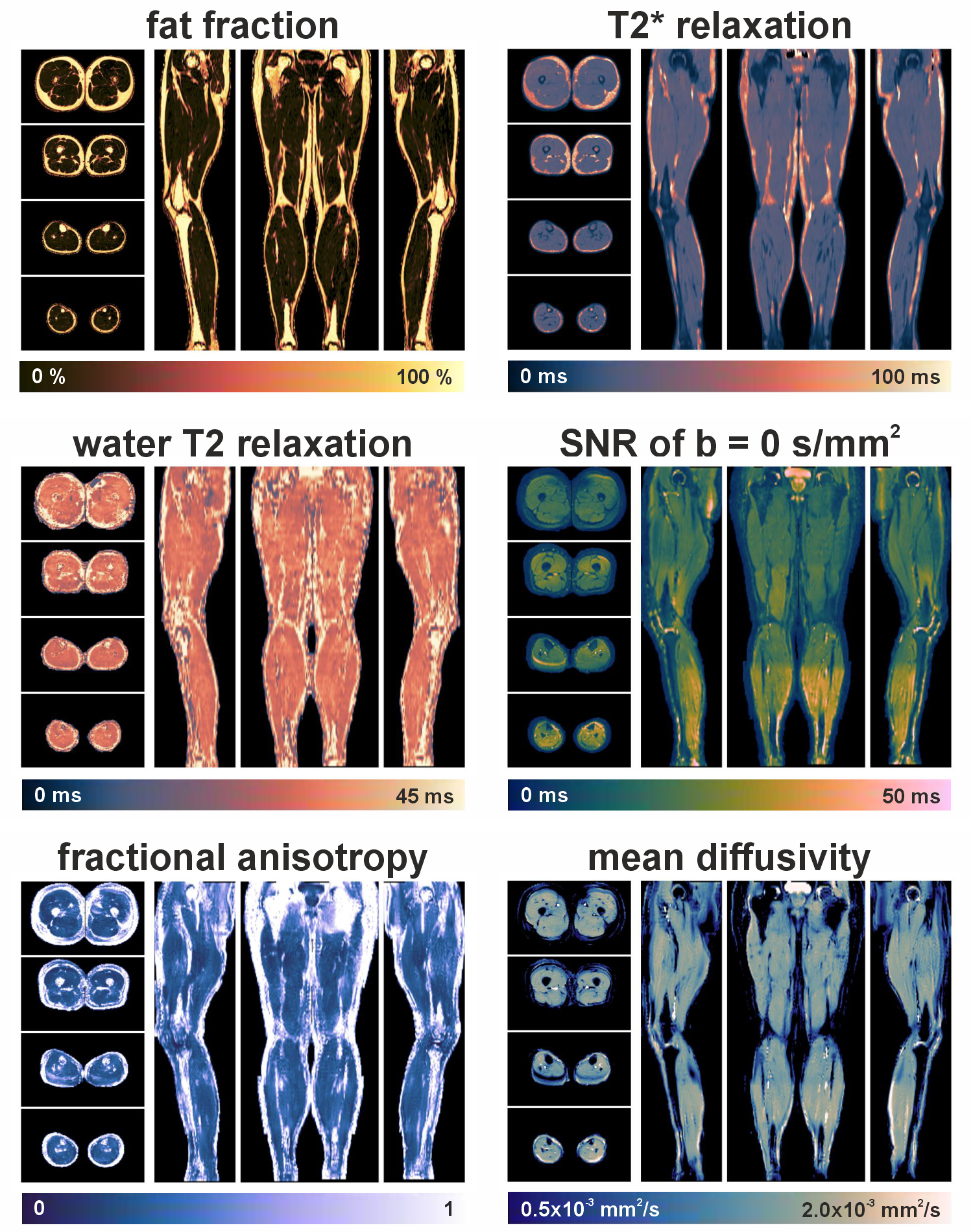
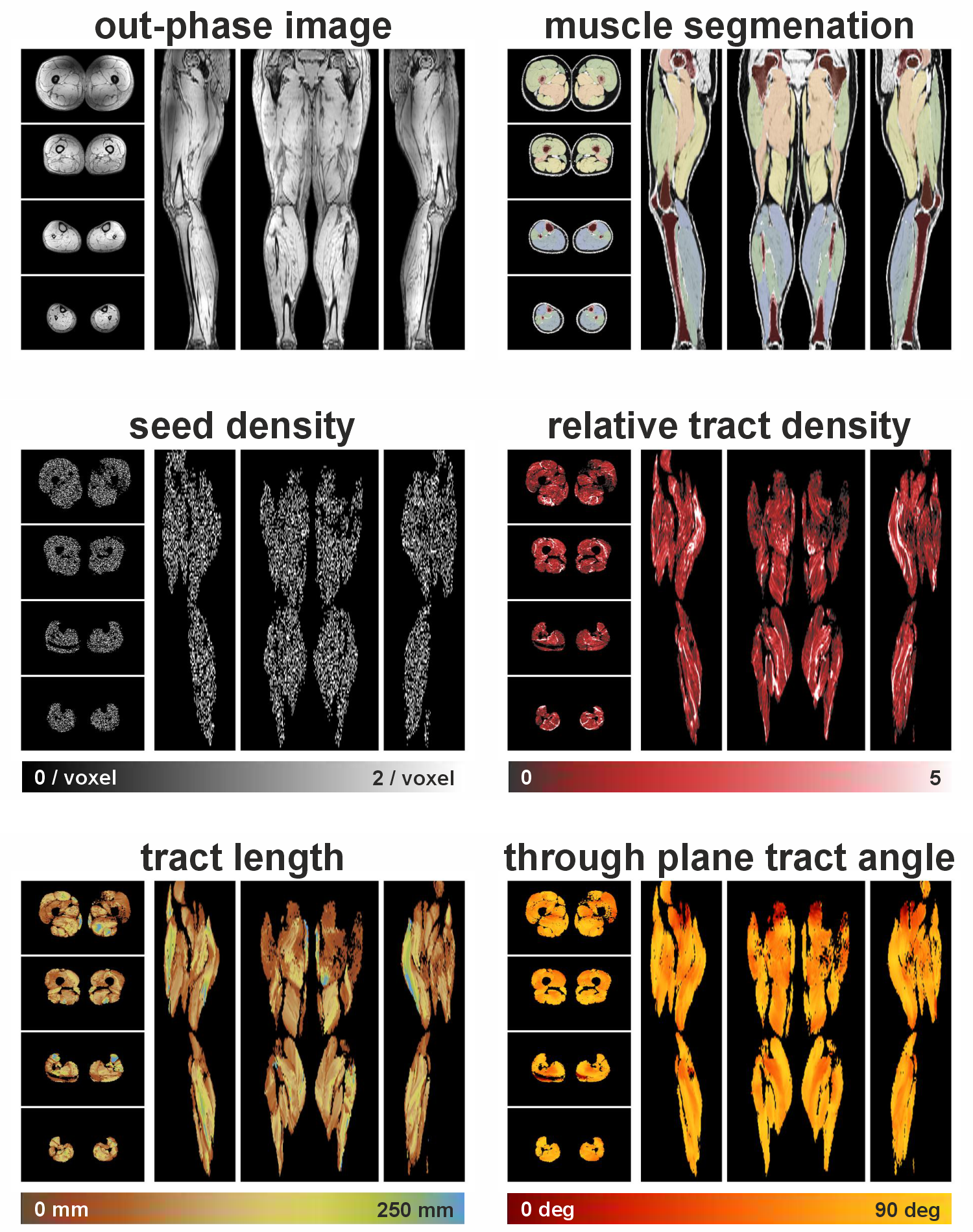
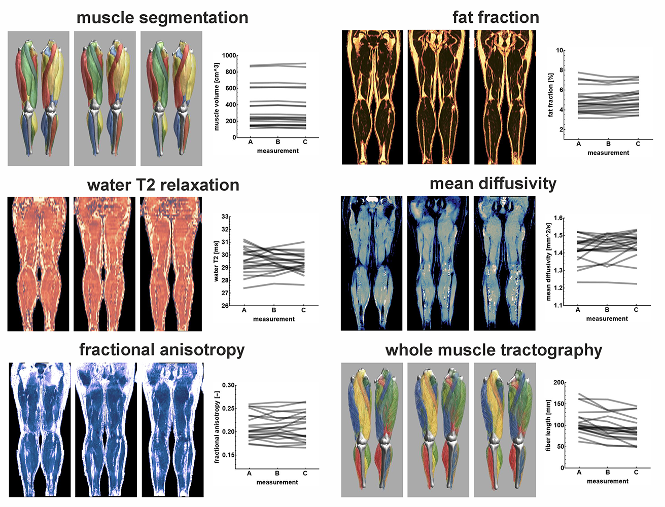
The pipeline was configured to produce merged full-leg quantitative maps (Figure 3) for the following data types: ME-GRE: in-phase and out-of-phase data, water and fat images, water and fat fractions, and T2* maps; ME-SE: water and fat images, water and fat-only T2 maps, water and fat fractions; SE-EPI: SNR, eigenvalue, RD, MD, and FA maps, IVIM perfusion fraction, and the tensor and b=0 s/mm² images. Additionally, from the fiber tractography seed, tract density, fiber length, and angle maps were derived (Figure 4). Results from three repeated scans of the same subject (with 3 months in between) are presented in Figure 5.Discussion and Conclusion
In this work, we have introduced a fully automated pipeline for processing and analyzing bilateral whole-leg multimodal qMRI data. While similar versatile pipelines exist, our pipeline distinguishes itself by its capability to process any number of overlapping stacks for multiple MRI contrasts, whether for unilateral or bilateral data. Moreover, it incorporates automated muscle segmentation and full-leg fiber tractography without requiring user interaction. Automated processing using open-source code is crucial for scaling study cohorts, ensuring result reproducibility, and facilitating the comparison of methods, tools, and data.Acknowledgements
No acknowledgement found.References
1. Strijkers GJ, Araujo ECA, Azzabou N, et al.: Exploration of new contrasts, targets, and MR imaging and spectroscopy techniques for neuromuscular disease-A workshop report of working group 3 of the biomedicine and molecular biosciences COST action BM1304 MYO-MRI. J Neuromuscul Dis 2019; 6:1–30.
2. Froeling M: QMRTools: a Mathematica toolbox for quantitative MRI analysis. J Open Source Softw 2019; 4:1204.
3. Yu H, McKenzie CA, Shimakawa A, et al.: Multiecho reconstruction for simultaneous water-fat decomposition and T2* estimation. Journal of Magnetic Resonance Imaging 2007; 26:1153–1161.
4. Bydder M, Yokoo T, Yu H, Carl M, Reeder SB, Sirlin CB: Constraining the initial phase in water-fat separation. Magn Reson Imaging 2011; 29:216–221.
5. Peterson P, Månsson S: Simultaneous quantification of fat content and fatty acid composition using MR imaging. Magn Reson Med 2013; 69:688–697.
6. Keene KR, Beenakker JWM, Hooijmans MT, et al.: T2 relaxation-time mapping in healthy and diseased skeletal muscle using extended phase graph algorithms. Magn Reson Med 2020; 84:2656–2670.
7. Marty B, Baudin PY, Reyngoudt H, et al.: Simultaneous muscle water T2 and fat fraction mapping using transverse relaxometry with stimulated echo compensation. NMR Biomed 2016; 29:431–443.
8. Collier Q, Veraart J, Jeurissen B, Den Dekker AJ, Sijbers J: Iterative reweighted linear least squares for accurate, fast, and robust estimation of diffusion magnetic resonance parameters. Magn Reson Med 2015; 73:2174–2184.
9. Veraart J, Novikov DS, Christiaens D, Ades-aron B, Sijbers J, Fieremans E: Denoising of diffusion MRI using random matrix theory. Neuroimage 2016; 142:394–406.
10. Tax CMW, Otte WM, Viergever MA, Dijkhuizen RM, Leemans A: REKINDLE: Robust Extraction of Kurtosis INDices with Linear Estimation. Magn Reson Med 2015; 73:794–808.
11. De Luca A, Bertoldo A, Froeling M: Effects of perfusion on DTI and DKI estimates in the skeletal muscle. Magn Reson Med 2017; 78:233–246.
12. Froeling M, Oudeman J, Strijkers GJ, et al.: Muscle changes detected with diffusion-tensor imaging after long-distance running. Radiology 2015; 274:548–562.
13. Ronneberger O, Fischer P, Brox T: U-net: Convolutional networks for biomedical image segmentation. Lecture Notes in Computer Science (including subseries Lecture Notes in Artificial Intelligence and Lecture Notes in Bioinformatics) 2015; 9351:234–241.
14. Rohm M, Markmann M, Forsting J, Rehmann R, Froeling M, Schlaffke L: 3D Automated Segmentation of Lower Leg Muscles Using Machine Learning on a Heterogeneous Dataset. Diagnostics 2021; 11:1–15.
Figures