2253
Learned Variable Flip-Angles to Improve Bi-Exponential 3D T2 and T1rho Mapping on the Knee Cartilage1Bernard and Irene Schwartz Center for Biomedical Imaging, Department of Radiology, New York University Grossman School of Medicine, New York, NY, United States, 2Center for Advanced Imaging Innovation and Research (CAI2R), Department of Radiology, New York University Grossman School of Medicine, New York, NY, United States, 3Siemens Medical Solutions, Malvern, PA, United States
Synopsis
Keywords: Cartilage, Quantitative Imaging
Motivation: Bi-exponential T2 and T1rho mapping of the knee cartilage can potentially improve early detection of knee osteoarthritis.
Goal(s): Scan time is usually long and SNR is low with standard methods. We plan to improve these aspects with a machine-learned pulse sequence.
Approach: We use a machine learning approach, called optimized variable flip-angles (OVFA) on magnetization-prepared gradient-echo (MPGRE) sequences to improve bi-exponential T2 and T1rho mapping on the knee cartilage.
Results: We observed an improvement of ~50% in SNR and a reduction of acquisition time by almost 2X when compared to standard MAPSS, typically used for quantitative T1rho and T2 mapping.
Impact: This study shows that the learned pulse sequence, named MPGRE-OVFA, can obtain similar bi-exponential T2 and T1rho mapping values as MAPSS, but it is 2 times faster and has 50% more SNR, potentially improving early detection of osteoarthritis.
Introduction:
High SNR and short scan time are important properties of MRI pulse sequences used for quantitative mapping, particularly bi-exponential (BE) T2 and T1rho mapping for early detection of osteoarthritis (OA) (1). We demonstrate the potential of using machine learning methods to improve magnetization-prepared gradient-echo (MPGRE) sequences (2–4) by optimizing the flip-angles (FA) individually (5). We compare the proposed sequence against one of the standard sequences for T1rho mapping, the magnetization-prepared angle-modulated partitioned k-space spoiled GRE snapshots (MAPSS) (2,6). The proposed sequence, named MPGRE-OVFA (from optimized variable flip-angles) is nearly 2X faster and achieves 50% better SNR than MAPSS, being 2X more SNR efficient.Methods:
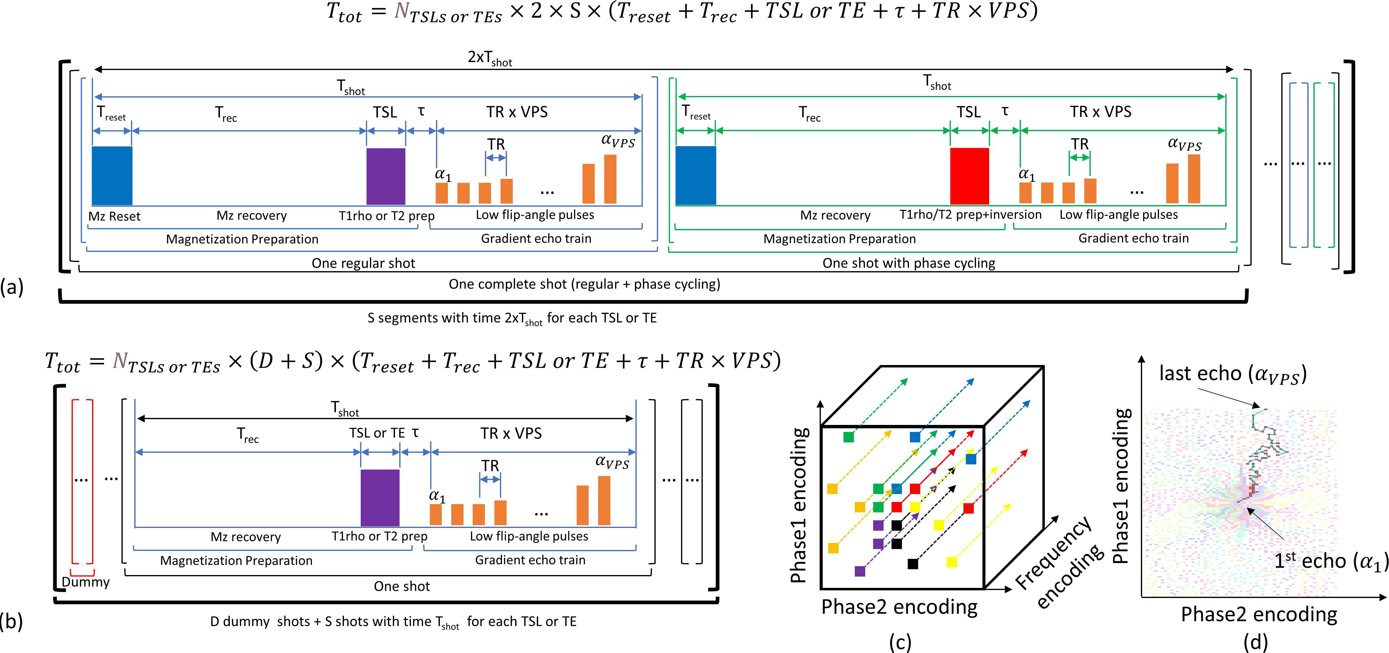
Sequences MAPSS (6) and MPGRE (7) used for T2 and T1rho mapping are shown in Figure 1(a) and 1(b) respectively, with their total time ($$$T_{tot}$$$). MAPSS is accurate because it uses Mz-reset pulse at each shot, followed by Mz recovery (Trec), T1rho or T2 preparation, and an imaging echo train that acquires several k-space lines. It uses phase-cycling shots to remove T1 contamination. The number of lines collected, or views-per-segment (VPS), and its center-out ordering (8) are shown in Figures 1(c) and (d). Fully sampled or undersampled patterns may be used (8,9). MPGRE is simpler, it does not use Mz-reset pulse or phase-cycling shots, which allows for much smaller Trec and faster scans. MPGRE may require some dummy shots (where no data is acquired) to reach a steady state. MAPSS uses optimized FA to reduce filtering effects (6). MPGRE typically uses constant FA and it is less accurate than MAPSS (7). However, with the machine learning framework from (5), a variable FA is learned not only to reduce filtering effects (10), but also to improve SNR and accuracy, correcting T1 contamination by adjusting the FAs. This results in a sequence as accurate as MAPSS but faster and with better SNR.The equations used for the signal evolution (SE) model for MPGRE and MAPSS sequences are described in (5). We learned the FA using:
$${\bf \hat{\alpha}}=\arg\min_{\alpha}\left[\sum_{k=1}^K\omega_k\left(\lambda_A||{\bf Am}_k(\alpha)||_2^2+\lambda_F||{\bf Fm}_k(\alpha)||_2^2+\lambda_S||{\bf S}({\bf m}_k(\alpha)-{\bf m}_{ref}||_2^2 \right)\right]$$
where $$${\bf m}_k(\alpha)$$$ in the normalized SE, $$${\bf m}_k(\alpha)=[M_{xy}(k,t_1,1,1)/e^{-\frac{t_1}{T_{1\rho}(k)}}...M_{xy}(k,t_T,S+D,VPS)/e^{-\frac{t_T}{T_{1\rho}(k)}}]$$$, being $$$M_{xy}(k,t,s,n)$$$ the SE with relaxation set $$$1\leq k\leq K$$$, where $$$K$$$ is the number of relaxation sets, considering given relaxation values $$$T_{1}(k),T_{2}(k),T_{1\rho}(k)$$$, for $$$1\leq t\leq T$$$, where $$$T=N_{TLSs}$$$ or $$$T=N_{TEs}$$$ is the number of TSLs or TEs, on the shot $$$1\leq s\leq S+D$$$, after the flip-angle pulse $$$1\leq n\leq VPS$$$.
We used $$$\omega_k=|T_{1\rho}(k)|^2/\sum_{i=1}^{K}|T_{1\rho}(i)|^2$$$. The first term targets accuracy, with the matrix $$$\bf A$$$ computes the finite difference between all pairs of $$$M_{xy}(k,t_p,s,1)/e^{-\frac{t_T}{T_{1\rho}(k)}}$$$ and $$$M_{xy}(k,t_q,s,1)/e^{-\frac{t_T}{T_{1\rho}(k)}}$$$, being $$$t_p$$$ and $$$t_q$$$ two different TSLs\TEs. The second term reduces the filtering effects, where the matrix $$$\bf F$$$ computes the finite difference on the SE inside the shot. The third term targets a better SNR, where $$${\bf m}_{ref}$$$ is the reference signal, and the matrix $$${\bf S}$$$ has ones in the positions we want to be close to $$${\bf m}_{ref}$$$, and zeros on the others (see more in (5)).
The learning approach is weighted to achieve the same accuracy as MAPSS but with better SNR. This configuration helps to produce BE maps as accurately as possible while keeping the MPGRE advantage of better SNR.
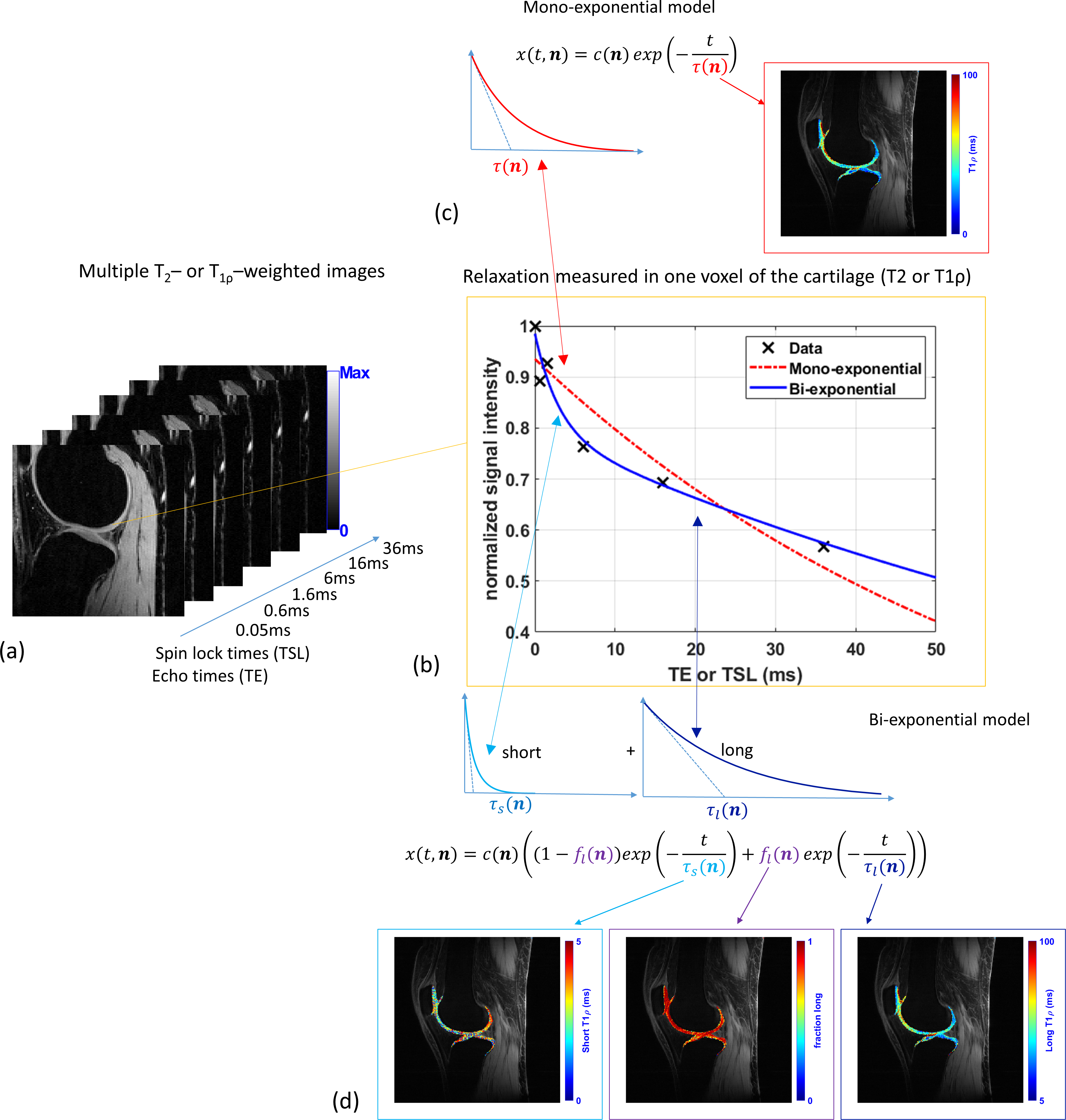
Mono-exponential (ME) and BE models are illustrated in Figure 2. The BE model includes the long component, short component, and their fraction. TSLs/TEs used in the magnetization-preparation step were: 0.05/0.6/1.6/6/16/36 ms. This selection is based on (11).
We scanned n=6 healthy volunteers. All scans were fully sampled and reconstructed with SENSE (12), and coil sensitivities from (13). ME and BE fitting was performed with non-linear least squares, using complex-valued voxels, and was minimized with the TRCG method (14). We compute the central tendency of ROI values using robust estimation (15) using median ±1.48xMAD (median of absolute deviation).
Results:
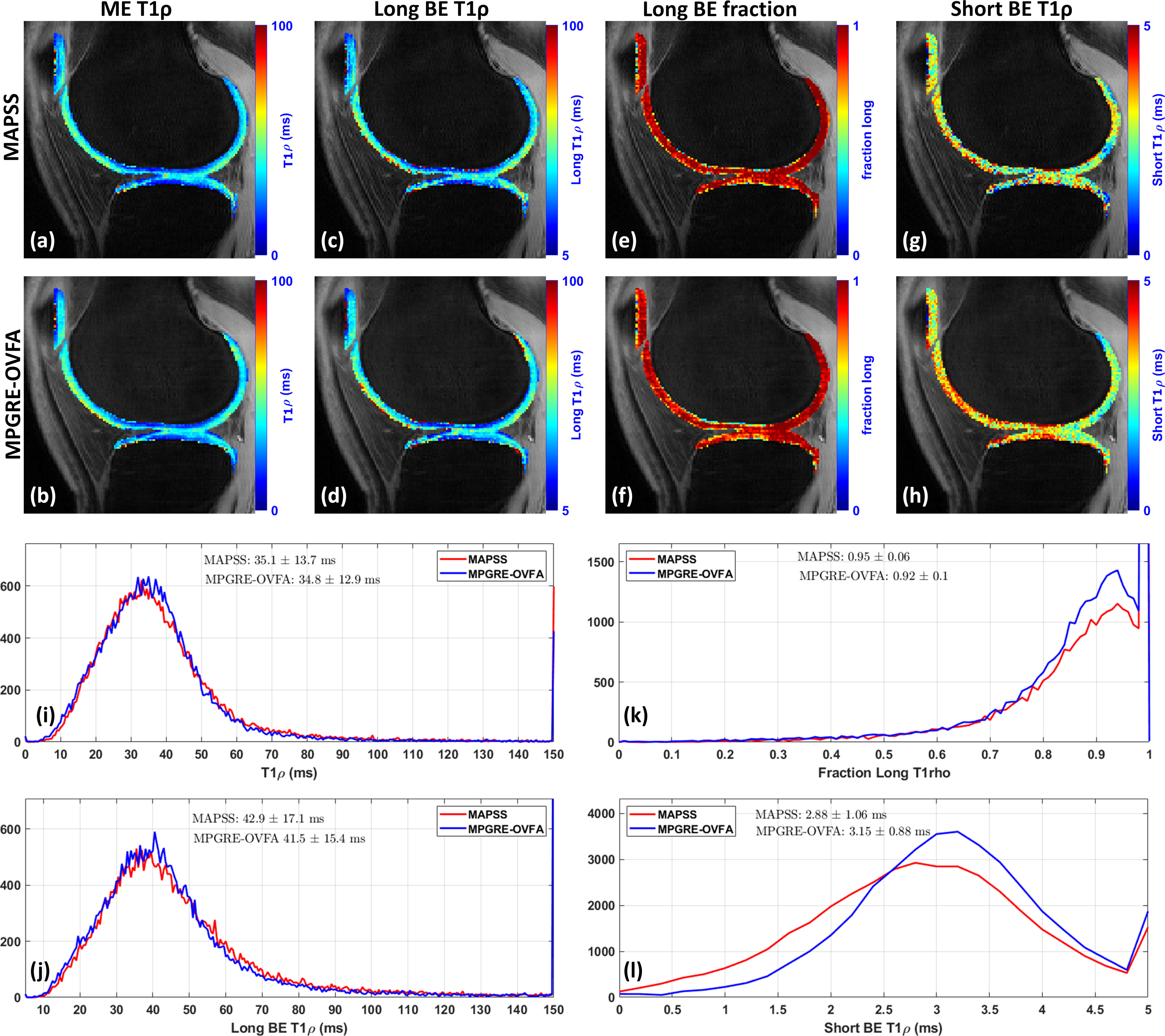
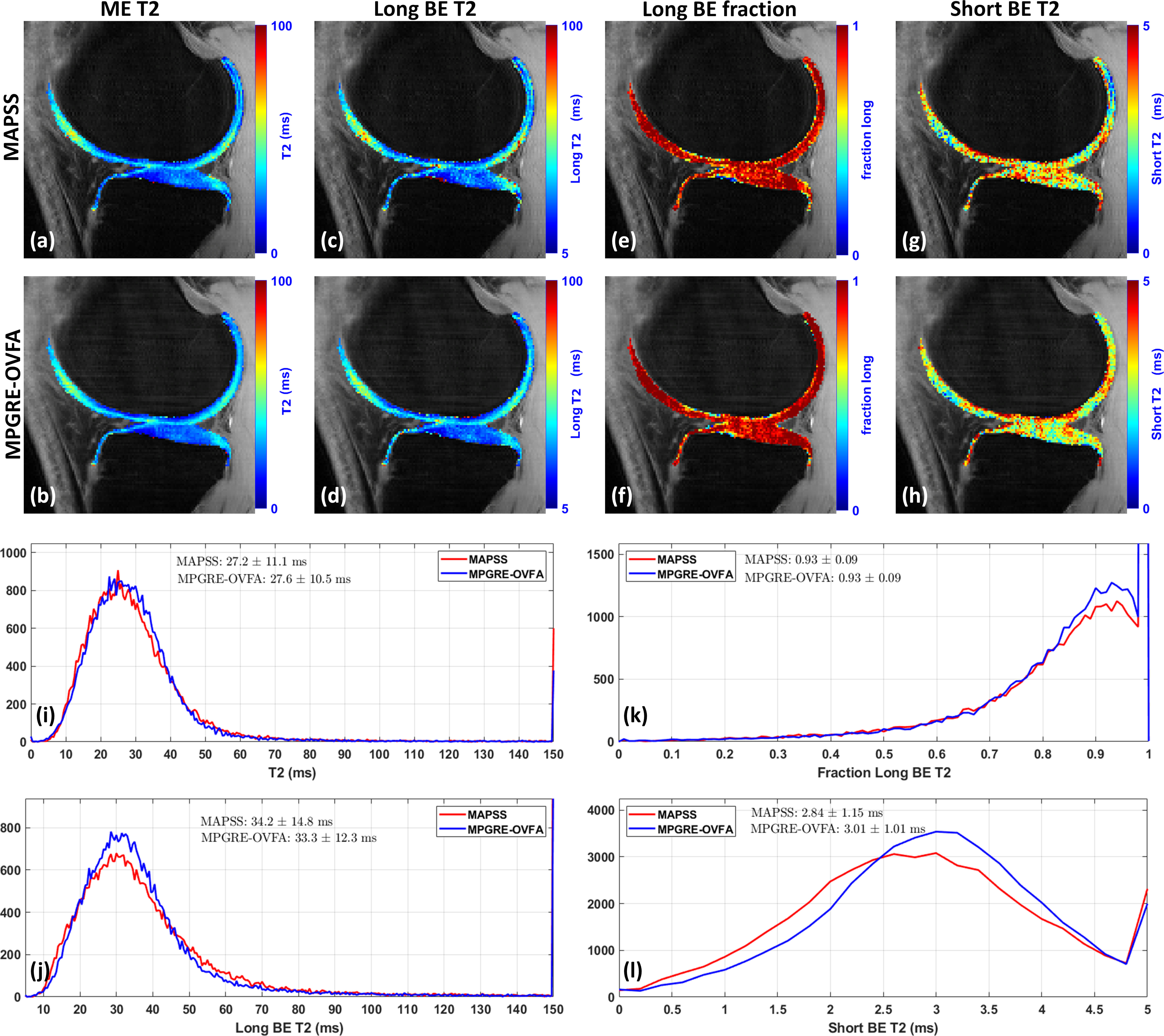
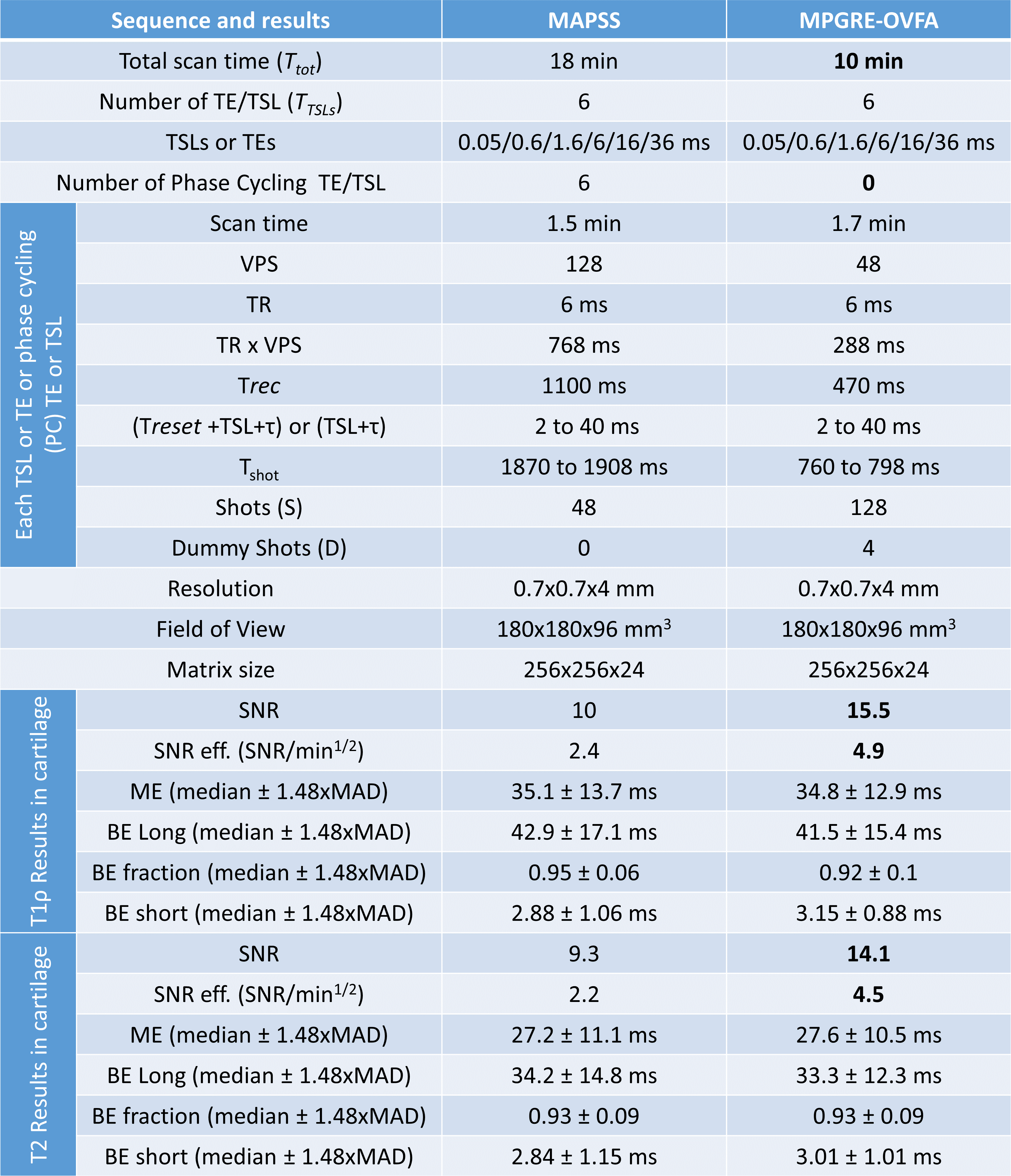
Visual results for T1rho and T2 mapping of knee cartilage are shown in Figures 3 and 4 respectively. Histograms of voxel-wise values in the cartilage for all volunteers are also shown. Table 1 shows the pulse sequence parameters, scan times, SNR, and relaxation values in the knee cartilage.Discussion and Conclusion:
The learned sequence, MPGRE-OVFA was able to obtain similar T2 and T1rho values as MAPSS, only with a little less dispersion, likely due to better SNR. The learned sequence is almost twice as fast as MAPSS. This is important for BE mapping on OA research, where 3D maps produced with fully sampled k-space data can be obtained in around 10 minutes with good SNR. In the future, learned sequences can replace traditional ones, with much shorter scan times and better SNR.Acknowledgements
This study was supported by NIH grantsR01-AR076328-01A1, R01-AR076985-01A1, and R01-AR078308-01A1 and was performed under the rubric of the Center of Advanced Imaging Innovation and Research (CAI2R), an NIBIB Biomedical Technology Resource Center (NIH P41-EB017183). Matlab codes for this work are available at https://cai2r.net/resources/ovfa-mp-gre/.References
1. Zibetti MVW, Menon RG, de Moura HL, Zhang X, Kijowski R, Regatte RR. Updates on Compositional MRI Mapping of the Cartilage: Emerging Techniques and Applications. J. Magn. Reson. Imaging 2023:1–17 doi: 10.1002/jmri.28689.
2. Peng Q, Wu C, Kim J, Li X. Efficient phase‐cycling strategy for high‐resolution 3D gradient‐echo quantitative parameter mapping. NMR Biomed. 2022;35:1–19 doi: 10.1002/nbm.4700.
3. He L, Wang J, Lu Z-L, Kline-Fath BM, Parikh NA. Optimization of magnetization-prepared rapid gradient echo (MP-RAGE) sequence for neonatal brain MRI. Pediatr. Radiol. 2018;48:1139–1151 doi: 10.1007/s00247-018-4140-x.
4. Hargreaves B. Rapid gradient‐echo imaging. In: Journal of Magnetic Resonance Imaging. Vol. 36. ; 2012. pp. 1300–1313. doi: 10.1002/jmri.23742.
5. Zibetti MVW, De Moura HL, Keerthivasan MB, Regatte RR. Optimizing variable flip angles in magnetization‐prepared gradient‐echo sequences for efficient 3D‐T1ρ mapping. Magn. Reson. Med. 2023;90:1465–1483 doi: 10.1002/mrm.29740.
6. Li X, Han ET, Busse RF, Majumdar S. In vivo T1ρ mapping in cartilage using 3D magnetization-prepared angle-modulated partitioned k-space spoiled gradient echo snapshots (3D MAPSS). Magn. Reson. Med. 2008;59:298–307 doi: 10.1002/mrm.21414.
7. Sharafi A, Xia D, Chang G, Regatte RR. Biexponential T 1ρ relaxation mapping of human knee cartilage in vivo at 3 T. NMR Biomed. 2017;30:e3760 doi: 10.1002/nbm.3760.
8. Zibetti MVW, Sharafi A, Keerthivasan MB, Regatte RR. Prospective Accelerated Cartesian 3D-T1rho Mapping of Knee Joint using Data-Driven Optimized Sampling Patterns and Compressed Sensing. In: Proceedings of the Annual Meeting of ISMRM 2021. ; 2021.
9. Zibetti MVW, Herman GT, Regatte RR. Fast data-driven learning of parallel MRI sampling patterns for large scale problems. Sci. Rep. 2021;11:19312 doi: 10.1038/s41598-021-97995-w.
10. Zhu D, Qin Q. A revisit of the k-space filtering effects of magnetization-prepared 3D FLASH and balanced SSFP acquisitions: Analytical characterization of the point spread functions. Magn. Reson. Imaging 2022;88:76–88 doi: 10.1016/j.mri.2022.01.015.
11. de Moura HL, Menon RG, Zibetti MVW, Regatte RR. Optimization of spin-lock times for T1ρ mapping of human knee cartilage with bi- and stretched-exponential models. Sci. Rep. 2022;12:16829 doi: 10.1038/s41598-022-21269-2.
12. Pruessmann KP, Weiger M, Scheidegger MB, Boesiger P. SENSE: Sensitivity encoding for fast MRI. Magn. Reson. Med. 1999;42:952–962 doi: 10.1002/(SICI)1522-2594(199911)42:5<952::AID-MRM16>3.0.CO;2-S.
13. Uecker M, Lai P, Murphy MJ, et al. ESPIRiT-an eigenvalue approach to autocalibrating parallel MRI: Where SENSE meets GRAPPA. Magn. Reson. Med. 2014;71:990–1001 doi: 10.1002/mrm.24751.
14. Steihaug T. The conjugate gradient method and trust regions in large scale optimization. SIAM J. Numer. Anal. 1983;20:626–637 doi: 10.1137/0720042.
15. Huber P, Ronchetti E. Robust statistics. 1981.
Figures