2251
In vivo T1 and T2 mapping of human knee at 0.05 Tesla1Laboratory of Biomedical Imaging and Signal Processing, The University of Hong Kong, Hong Kong SAR, China, 2Department of Electrical and Electronic Engineering, The University of Hong Kong, Hong Kong SAR, China
Synopsis
Keywords: Cartilage, Low-Field MRI, T2 mapping, T1 mapping
Motivation: To study knee tissue properties at Ultra-low-field (ULF) for sequence design/optimization, enabling ULF MRI for wide-ranging applications.
Goal(s): To measure the T2 and T1 values of various tissues in vivo human knee at 0.05T.
Approach: Multiple TE and TR measurements were conducted on a home-built and RF shielding-free 0.05T MRI scanner for T2 and T1 mapping through pixel-wise numerical fitting.
Results: Phantom results exhibited a linear relationship between the Gadolinium concentration and relaxation rate, demonstrating the feasibility of mapping procedure. Additionally, the T2 and T1 values of cartilage, tendon, fat, and skeletal muscle in human knee were estimated and reported.
Impact: The estimated Gadolinium T2 and T1 relaxivities at 0.05 Tesla are significantly higher than those at 1.5T and 3.0T, guiding the usage of contrast agent dose. Moreover, T2 and T1 mapping of musculoskeletal tissues can facilitate sequence design/optimization.
Introduction
Ultra-low-field (ULF) MRI is a promising way to enhance global healthcare accessibility due to its low cost, low power consumption, and small footprint1-4. To achieve the desired image contrasts at ULF, tissue properties, i.e., T2 and T1 values, are necessary for sequence design/optimization. Meanwhile, measurement of tissue T2 and T1 values can provide unbiased information regardless of scan parameters5. However, the T2 and T1 values of musculoskeletal tissues, i.e., human knee, remain unknown at ULF. In this study, we first conduct T2 and T1 mapping of Gadolinium (Gd)-doped water phantoms to validate the feasibility of the procedure, and then map the T2 and T1 values of human knee on a low-cost and shielding-free 0.05T ULF MRI scanner.Method
Sequences for T2 and T1 mappingT2 mapping was conducted using 3D multi-echo FSE sequence with sixteen TEs (ESP=18ms), TR = 500ms, and total acquisition time = 14 minutes. T1 mapping was conducted using 3D SE sequences with different TRs of 50, 75, 100, 150, 200, and 300ms, TE =18ms, and total acquisition time = 25.2 minutes. Other scan parameters were the same: bandwidth = 12.5kHz, acquisition resolution = 2×2×8mm3, matrix size = 108×108×16, and NEX = 1.
Phantom and in vivo experiments
All experiments were conducted on a home-built permanent magnet based 0.05 Tesla MRI scanner using a self Tx/Rx knee coil. The scanner had a similar design to that reported in our previous work1, which was free from any magnetic and RF shielding. All scans were conducted using the above-mentioned sequences at a temperature around 24°C. Six Gd-doped water phantoms with different Gd concentrations (0.5, 1.0, 1.5, 2.0, 2.5 and 4.0mmol/L) were used to validate the mapping procedure. Afterward, four healthy subjects (male, aged 30±4 years) were enrolled under institutional review board approval with written informed consents. Knee images in sagittal view for T1 and T2 mapping were acquired using the above-mentioned sequences.
Data processing
K-space data were first processed for electromagnetic interference (EMI) signal removal by utilizing active EMI sensing and deep learning EMI signal prediction and cancellation1, without any EMI characterization data acquisition. Afterward, pixel-wise T1 and T2 mapping were performed after image reconstruction.
T1 mapping was conducted by fitting the acquired six image datasets with different TRi to the model: $$S_{i}=A\cdot(1-e^{-\frac{TR_{i} }{T1} } )+N$$ For T2 mapping, the acquired sixteen image datasets with different TEi were fitted to the model: $$S_{i}=A\cdot e^{-\frac{TE_{i} }{T2} }+N$$ In the above-mentioned two models, Si was the pixel signal intensity, N was the pre-estimated noise level, A was the signal amplitude, and T1 and T2 were the T1 and T2 relaxation times, respectively. ROIs were manually drawn to calculate the averaged T2 and T1 values for Gd-doped phantoms and in vivo knee tissues, including cartilage, tendon, skeletal muscle, subcutaneous fat and bone marrow fat.
Results
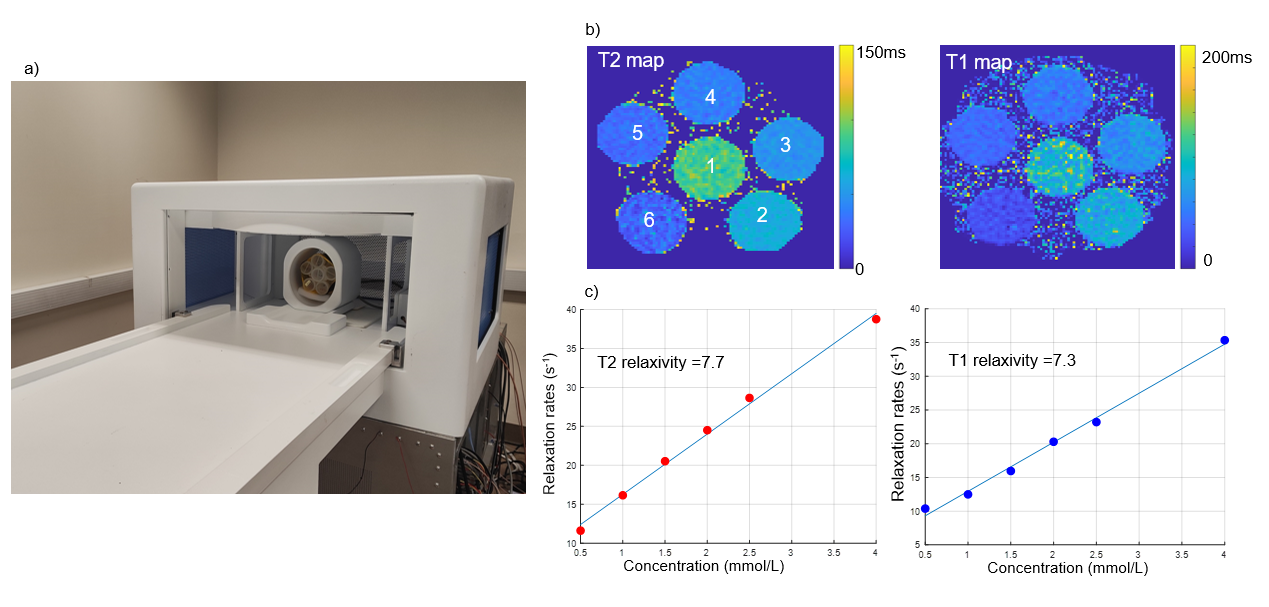
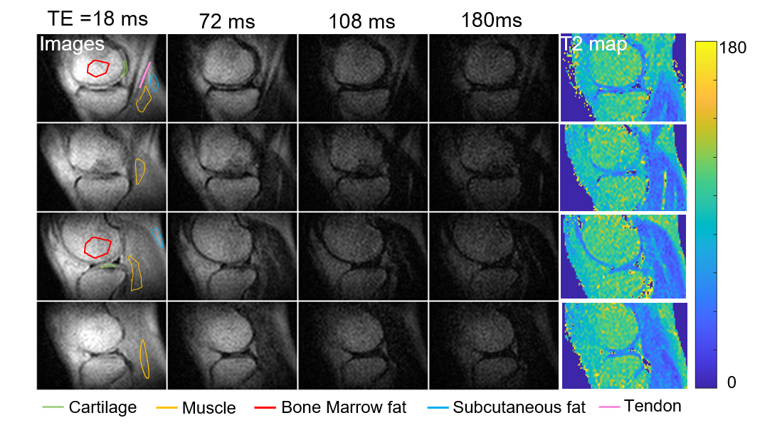
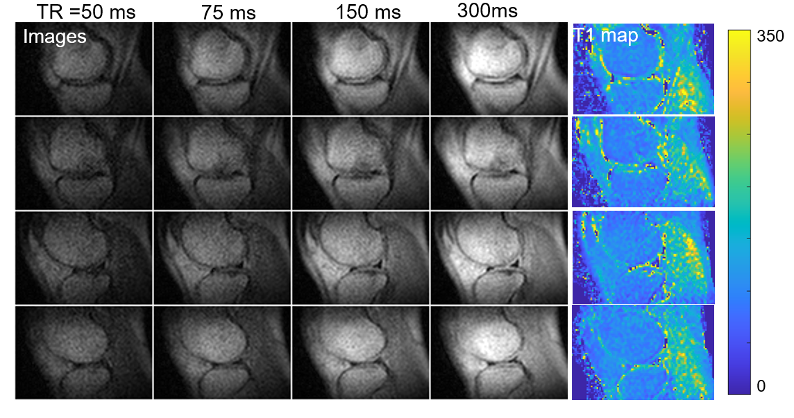
Figure 1 shows scan setup (Figure 1a) as well as the T2 and T1 mapping results of Gd-doped phantoms. Both the T2 and T1 values decrease with the increasing Gd concentrations (Figure 1b), and the T2 and T1 relaxation rates hold a linear relationship with the Gd concentration (Figure 1c). Moreover, the estimated T2 and T1 relaxivities are 7.7 and 7.3 L·mmol-1·s-1, respectively, which are significantly higher than those at high field (i.e., T2 and T1 relaxivities of 3.2 and 2.9 L·mmol-1·s-1 at 1.5T for the same contrast agent6). The measured T2 and T1 values are reported in Table 1.The representative knee images as well as T2 and T1 maps of one subject are shown in Figures 2 and 3, respectively. Different knee tissues can be readily distinguished from the raw images with adequate SNR, spatial resolution, and contrast (Figures 2 and 3). The measured T2 values of cartilage, tendon, subcutaneous fat, bone marrow fat, and skeletal muscle are 54.4ms, 54.1ms, 100.7ms, 104.6ms and 41.9ms, respectively (Figures 2 and Table 3). Regarding T1 mapping results, the estimated T1 values of cartilage, tendon, subcutaneous fat, bone marrow fat, and skeletal muscle are 218.5ms, 197.2ms, 120.5ms, 111.7ms and 188.9ms, respectively (Figures 2 and Table 3).
Discussion and Conclusions
In this study, T1 and T2 values of in vivo human knee tissues, including cartilage, tendon, skeletal muscle, and fat, were estimated at 0.05T even with low SNR and spatial resolution. T1 and T2 relaxivities of Gd contrast agent were measured and significantly higher than those at high filed. The results are valuable for sequence design/optimization in ULF MRI.Acknowledgements
This work was supported in part by Hong Kong Research Grant Council (R7003-19F, HKU17112120, HKU17127121, HKU17127022 and HKU17127523 to E.X.W).References
[1] Liu Y, Leong ATL, Zhao Y, Xiao L, Mak HKF, Tsang ACO, Lau GKK, Leung GKK, Wu EX. A low-cost and shielding-free ultra-low-field brain MRI scanner. Nat Commun 2021;12(1):7238.
[2] Yuen MM, Prabhat AM, Mazurek MH, Chavva IR, Crawford A, Cahn BA, Beekman R, Kim JA, Gobeske KT, Petersen NH, Falcone GJ, Gilmore EJ, Hwang DY, Jasne AS, Amin H, Sharma R, Matouk C, Ward A, Schindler J, Sansing L, de Havenon A, Aydin A, Wira C, Sze G, Rosen MS, Kimberly WT, Sheth KN. Portable, low-field magnetic resonance imaging enables highly accessible and dynamic bedside evaluation of ischemic stroke. Science Advances 2022;8(16):eabm3952.
[3] He Y, He W, Tan L, Chen F, Meng F, Feng H, Xu Z. Use of 2.1 MHz MRI scanner for brain imaging and its preliminary results in stroke. J Magn Reson 2020;319:106829.
[4] Mazurek MH, Cahn BA, Yuen MM, Prabhat AM, Chavva IR, Shah JT, Crawford AL, Welch EB, Rothberg J, Sacolick L, Poole M, Wira C, Matouk CC, Ward A, Timario N, Leasure A, Beekman R, Peng TJ, Witsch J, Antonios JP, Falcone GJ, Gobeske KT, Petersen N, Schindler J, Sansing L, Gilmore EJ, Hwang DY, Kim JA, Malhotra A, Sze G, Rosen MS, Kimberly WT, Sheth KN. Portable, bedside, low-field magnetic resonance imaging for evaluation of intracerebral hemorrhage. Nat Commun 2021;12(1):5119.
[5] Baudrexel S, Nöth U, Schüre J-R, Deichmann R. T1 mapping with the variable flip angle technique: A simple correction for insufficient spoiling of transverse magnetization. Magnetic Resonance in Medicine 2018;79(6):3082-3092.
[6] Rohrer M, Bauer H, Mintorovitch J, Requardt M, Weinmann HJ. Comparison of magnetic properties of MRI contrast media solutions at different magnetic field strengths. Invest Radiol 2005;40(11):715-724.
[7] Martirosian P, Boss A, Deimling M, Kiefer B, Schraml C, Schwenzer NF, Claussen CD, Schick F. Systematic variation of off-resonance prepulses for clinical magnetization transfer contrast imaging at 0.2, 1.5, and 3.0 tesla. Invest Radiol 2008;43(1):16-26.
[8] Gold GE, Han E, Stainsby J, Wright G, Brittain J, Beaulieu C. Musculoskeletal MRI at 3.0 T: Relaxation Times and Image Contrast. American Journal of Roentgenology 2004;183(2):343-351.
[9] O’Reilly T, Webb AG. In vivo T1 and T2 relaxation time maps of brain tissue, skeletal muscle, and lipid measured in healthy volunteers at 50 mT. Magnetic Resonance in Medicine 2022;87(2):884-895.
Figures
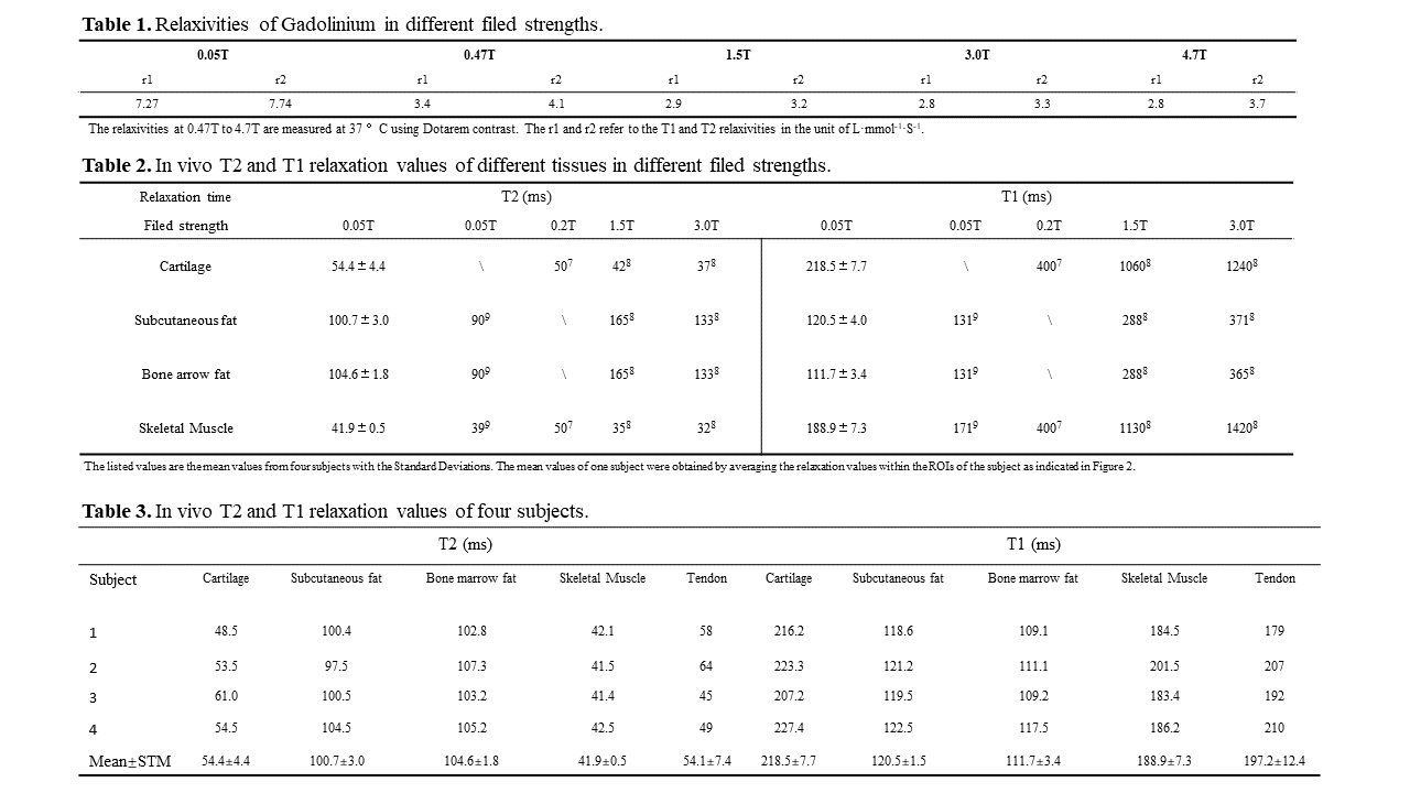
The tables of the relaxivities of Gadolinium in different filed strengths, T2 and T1 relaxation values of different tissues in different filed strengths, T2 and T1 relaxation values of four subjects.