2235

Comparison of Variational Autoencoders for Magnetic Resonance Spectroscopy Data Synthesis

Dennis van de Sande¹, Justin Kleinveld¹, Sina Amirrajab¹, Mitko Veta¹, and Marcel Breeuwer¹
¹Biomedical Engineering, Eindhoven University of Technology, Eindhoven, Netherlands

Synopsis

Keywords: Other AI/ML, Modelling, Generative modelling

Motivation: Scarcity of MRS datasets hinders deep learning model development, often leading to reliance on simulations which show difficulties with replicating in-vivo characteristics.

Goal(s): The goal is to evaluate different variational autoencoders to enhance MRS datasets and improve deep learning model development for MRS.

Approach: This study assesses different models for generating MRS data. Additionally, interpolation is done between multiple pairs of real spectra to improve the diversity of the synthetic data.

Results: One model shows great potential in terms of reconstruction quality and generative performance. The incorporation of interpolation further enhances the diversity in synthetic spectra, particularly in relation to residual water signals.

Impact: The demonstrated potential of variational autoencoders for MRS data generation will help in generating synthetic data that is similar to in-vivo data. This will help the development of other deep learning models for MRS applications.

Introduction

Deep learning (DL) has revolutionized medical imaging, enabling tasks like image reconstruction, denoising, segmentation, and classification¹. However, the need for extensive training datasets is a major challenge, often due to restricted access, high acquisition costs, and privacy concerns. Consequently, generative modeling techniques have emerged to address these limitations by augmenting small datasets with synthetic samples². Variational Autoencoders³(VAEs) are a type of probabilistic generative models utilizing an encoder-decoder architecture to learn a low-dimensional latent representation of the data. This latent representation can be used to generate new synthetic samples.

In the field of magnetic resonance spectroscopy (MRS), DL has become increasingly valuable for tasks like spectral denoising, artifact removal, and quantification⁴. Nevertheless, the scarcity of large MRS datasets hinders model development, often leading to reliance on simulated data. While physics-based MRS simulation models can be used for data generation, they cannot replicate in-vivo characteristics such as artifacts, lipid signals, and macromolecule signals. VAEs offer a promising solution to this challenge by generating synthetic data that is similar to in-vivo datasets in this respect.

This study aims to assess different VAE models for generating single-voxel MRS data, focusing on reconstruction quality and generative performance. The goal is to evaluate VAEs' potential to enhance MRS datasets and improve DL model development for MRS.

Materials and Methods

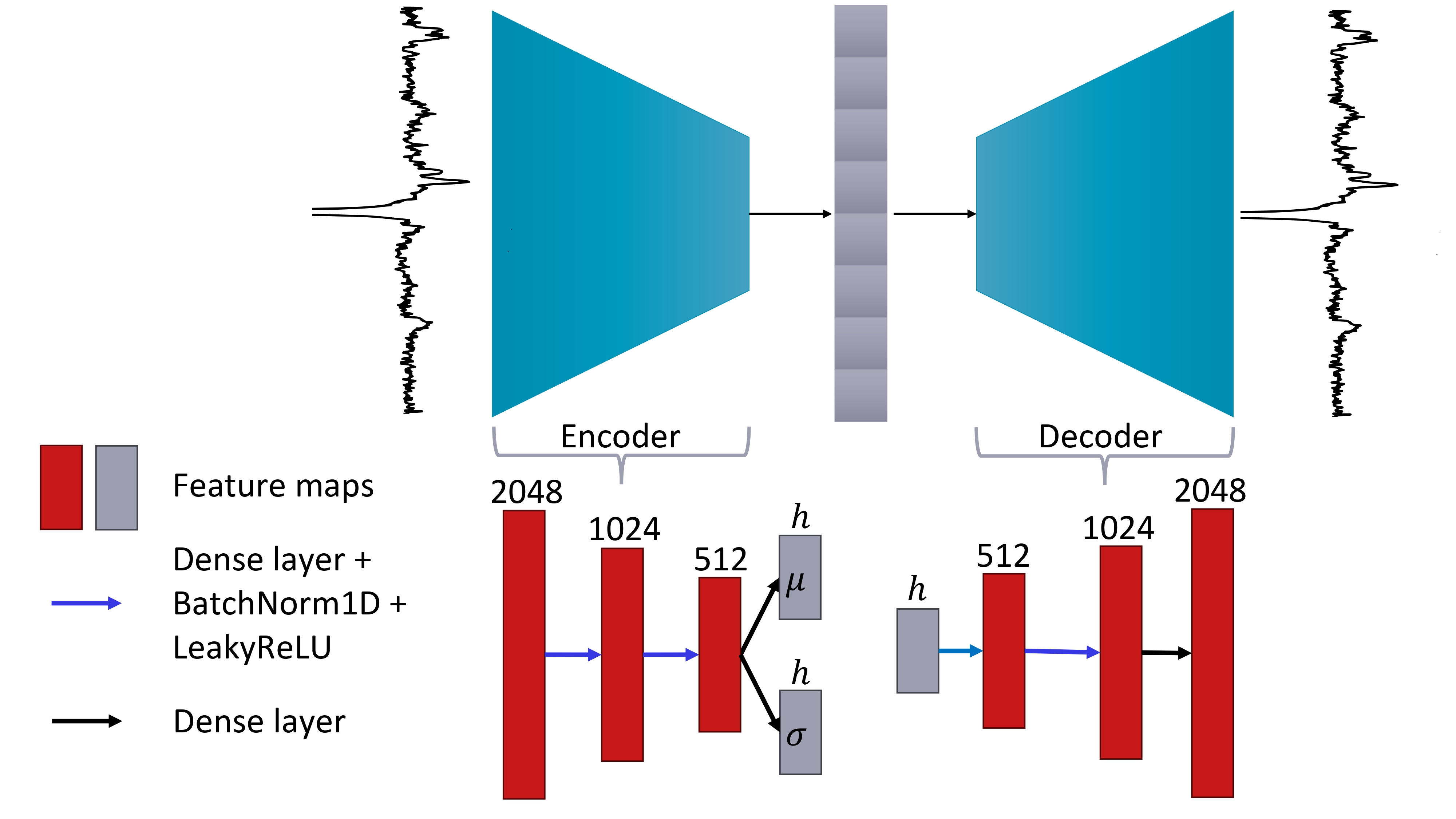
The dataset is derived from the ISBI Edited MRS Reconstruction Challenge's⁵ homogeneous in-vivo track, a subset of the Big-GABA dataset⁶. It includes data from GABA-edited MEGA-PRESS scans, featuring 12 patients with 160 ON and OFF transients, and 24 patients with 40 ON and OFF transients, each containing free induction decays (FIDs) with 2048 data points. Two datasets are created: one with individual transients and another with averages of 40 transients. Preprocessing includes Fourier transformation, ON and OFF spectrum subtraction, and normalization. Only the real part of the spectra is used, and the datasets are split into training, validation, and test sets, with respective splits of 2304/288/288 and 57/7/8 for the individual transient and the 40-transient average datasets.

Four different models are trained and compared: VAE³, β-VAE⁷, Information Maximizing VAE⁸ (Info-VAE), and Wasserstein Autoencoder⁹ (WAE). All models are implemented using the Pythae¹⁰ library with a custom 1D network architecture, which is shown in Figure 1. Where applicable, models are trained using the Mean Squared Error (MSE) reconstruction loss, the Kullback-Leibler loss (KL-loss), and the AdamW optimizer. Both the info-VAE and the WAE use the inverse multiquadratic kernel to calculate the maximum mean discrepancy. A random search is performed to find the optimal hyperparameters for each model.
The evaluation focuses on three components: reconstruction quality through MSE, qualitative evaluation, and feature comparison using t-distributed stochastic neighbor embedding (t-SNE). Additionally, we propose to perform interpolation between multiple pairs of real spectra in the latent space to improve the diversity of the synthetic data.

Results

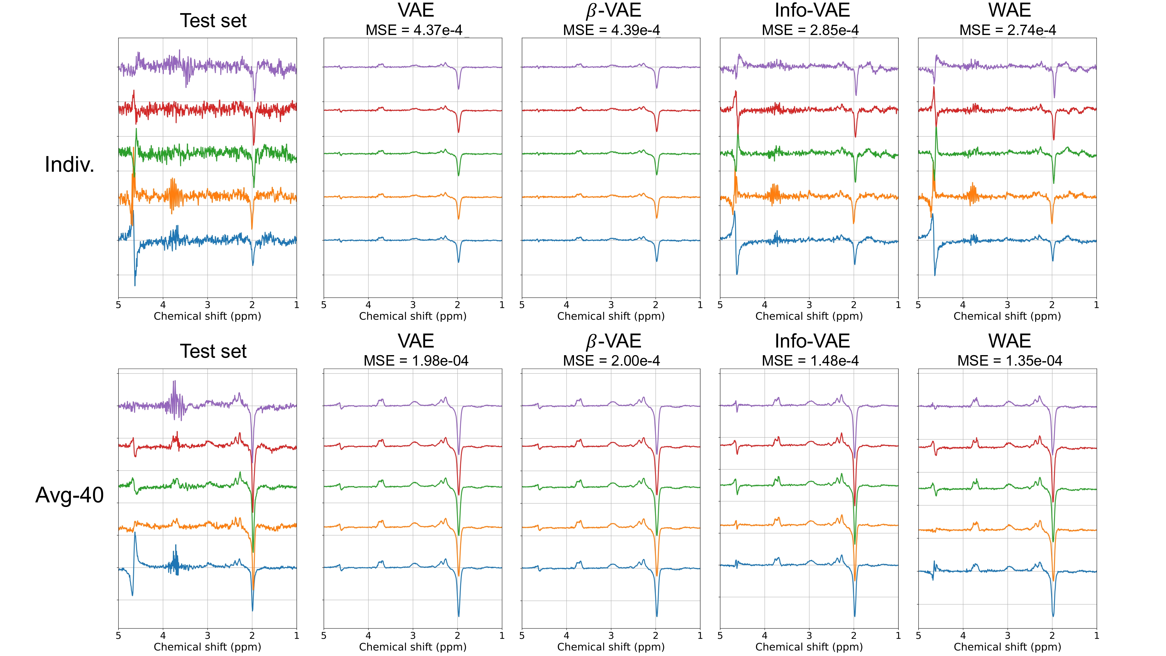
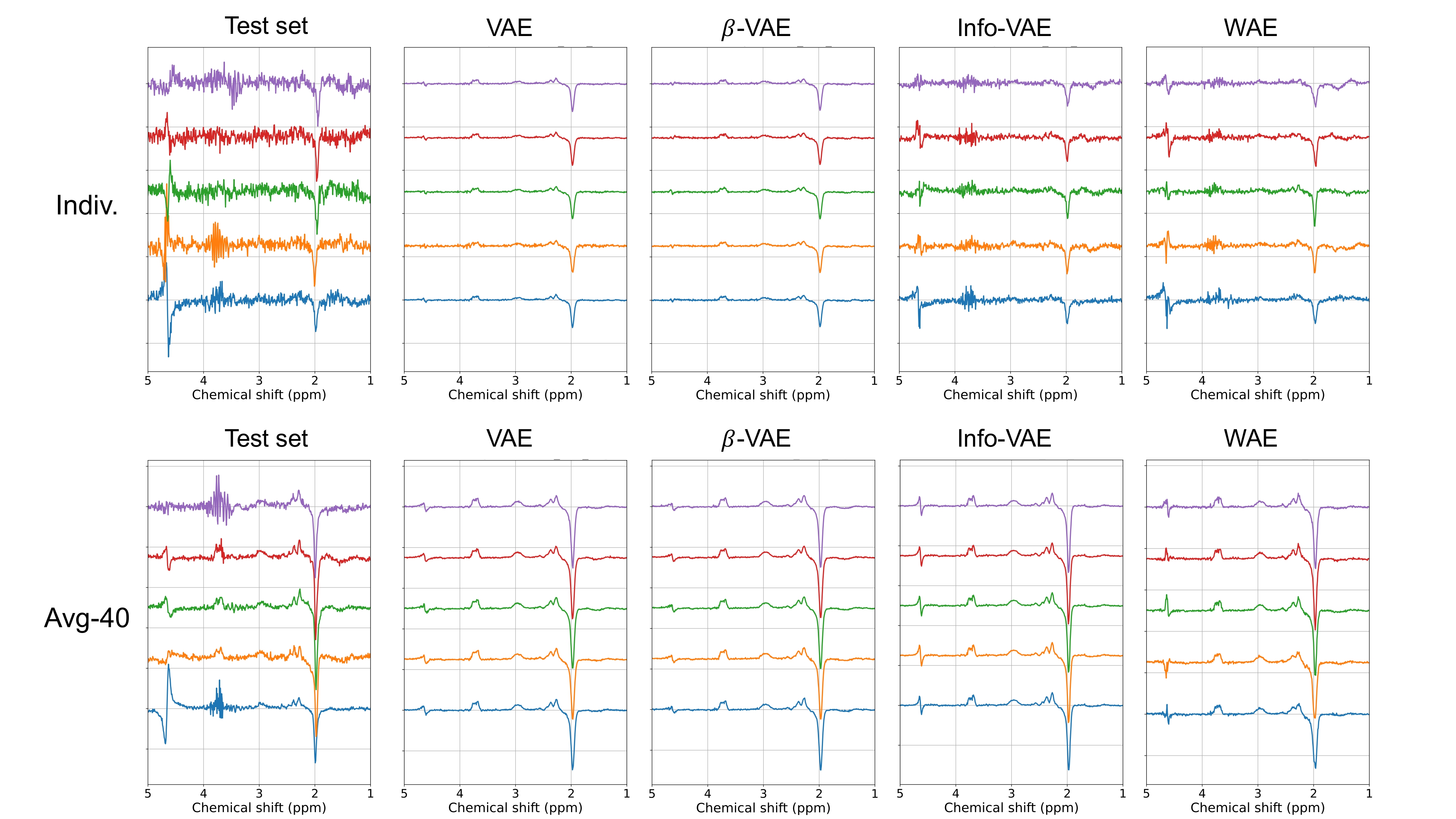
Figure 2 shows the reconstruction of five test spectra by all models, with noticeable noise reduction compared to the original test spectra. This effect is particularly prominent for the VAE and β-VAE reconstructions. In contrast, Info-VAE and WAE maintain some noise and excel in reconstructing the residual water signal (~4.6 ppm). Furthermore, the MSE scores demonstrate WAE's superior performance for both datasets.
Figure 3 showcases randomly generated spectra from each model. Notably, VAE and β-VAE-generated samples display reduced noise characteristics and residual water signal variations, consistent with observations in Figure 2.
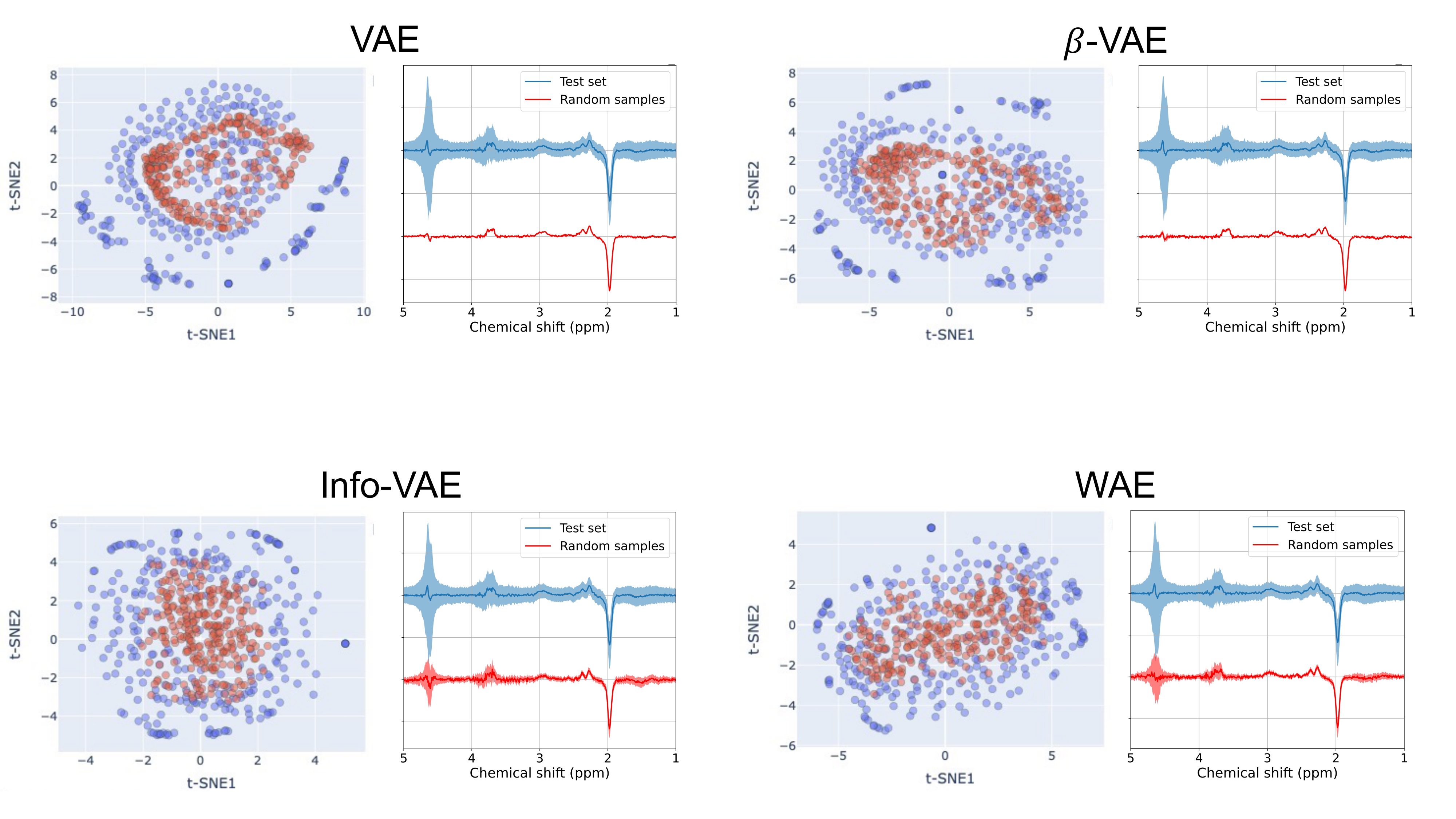
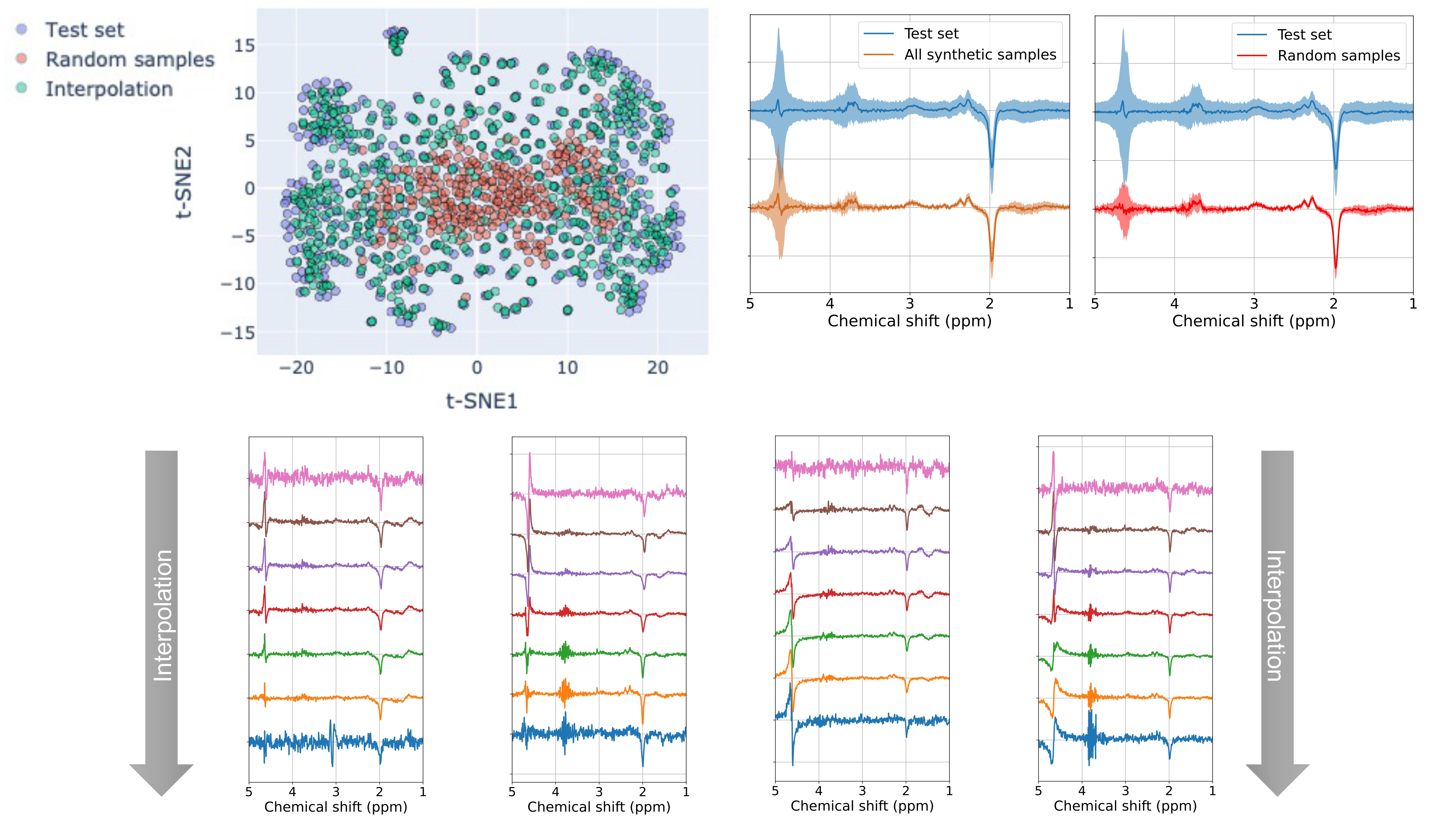
The t-SNE plots in Figure 4 are generated exclusively for the individual transient dataset due to limited number of samples in the 40-averaged transients. These plots reveal a distinct reduction in overlap between VAE and β-VAE samples compared to Info-VAE and WAE samples, suggesting that Info-VAE and WAE-generated spectra closely resemble test spectra.
Furthermore, examining the mean and standard deviation of the randomly generated samples in comparison to the test spectra, shows that the Info-VAE and WAE models exhibit the most substantial variation, with WAE performing slightly better.
Figure 5 presents the interpolation study for the top-performing model, WAE, which significantly increases diversity in synthetic spectra, particularly in relation to the residual water signal.

Discussion and Conclusion

This study highlights the potential of VAE models as generative tools for MRS data synthesis, with WAE excelling in reconstruction quality and generative performance. The t-SNE plots further confirm feature similarity between WAE-generated samples and real MRS data.
The incorporation of interpolation further enhances the diversity in synthetic spectra, particularly in relation to the residual water signal. Future directions employing these VAE models will focus on generating data for training DL applications, alongside leveraging latent space assessment and interpolation for artifact generation and removal.

Acknowledgements

This work was (partially) funded by Spectralligence (EUREKA IA Call, ITEA4 project 20209).

References

1. Chen X, Wang X, Zhang K, et al. Recent advances and clinical applications of deep learning in medical image analysis. Med Image Anal. 2022;79:102444. doi:10.1016/j.media.2022.102444

2. Kazeminia S, Baur C, Kuijper A, et al. GANs for medical image analysis. Artif Intell Med. 2020;109:101938. doi:10.1016/j.artmed.2020.101938

3. Kingma DP, Welling M. Auto-Encoding Variational Bayes. Published online May 1, 2014. doi:10.48550/arXiv.1312.6114

4. van de Sande, DMJ, Merkofer, JP, Amirrajab, S, et al. A review of machine learning applications for the proton MR spectroscopy workflow. Magn Reson Med. 2023; 90(4): 1253-1270. doi: 10.1002/mrm.29793

5. Berto RP, Bugler H, Dias G, et al. Advancing GABA-edited MRS Research through a Reconstruction Challenge. bioRxiv. Published online 2023. doi:10.1101/2023.09.21.557971

6. Mikkelsen M, Barker PB, Bhattacharyya PK, et al. Big GABA: Edited MR spectroscopy at 24 research sites. NeuroImage. 2017;159:32-45. doi:10.1016/j.neuroimage.2017.07.021

7. Higgins I, Matthey L, Pal A, et al. beta-VAE: Learning Basic Visual Concepts with a Constrained Variational Framework. In: International Conference on Learning Representations. ; 2017. https://openreview.net/forum?id=Sy2fzU9gl

8. Zhao S, Song J, Ermon S. InfoVAE: Information Maximizing Variational Autoencoders. arXiv [csLG]. Published online 2018. http://arxiv.org/abs/1706.02262

9. Tolstikhin I, Bousquet O, Gelly S, Schoelkopf B. Wasserstein Auto-Encoders. arXiv [statML]. Published online 2019. http://arxiv.org/abs/1711.01558

10. Chadebec C, Vincent L, Allassonnière S. Pythae: Unifying Generative Autoencoders in Python-A Benchmarking Use Case. Advances in Neural Information Processing Systems. 2022;35:21575-21589.

Figures

Figure 1: Schematic outline of the used model architecture for all VAEs. The structure is divided in an encoder and a decoder network. The encoder encodes the input to the latent space with latent dimension h. The decoder decodes the latent vector back to the original input size.

Figure 2: Visual comparison and Mean Squared Error (MSE) reconstruction scores on the test set for all models on both datasets. All reconstructions show denoised spectra compared to the test set, especially for the VAE and β-VAE reconstructions. In contrast, Info-VAE and WAE maintain some noise and excel in reconstructing the residual water signal (~4.6 ppm).

Figure 3: Visual comparison of randomly generated spectra for all models using both datasets. The same denoising effect is shown between the test set and the generated spectra. Info-VAE and WAE show larger variation in the residual water signal (~4.6 ppm), indicating better variability in the generated data.

Figure 4: T-SNE plots depicting all models using the individual transient dataset. Adjacent to the t-SNE plots, a graph displays the mean and standard deviation of both the test spectra and the randomly generated spectra. Info-VAE and WAE-generated spectra show a stronger alignment with the test set in the t-SNE plots, signifying a closer feature resemblance. Furthermore, the generated samples of these two models also demonstrate greater variation, with a slight advantage observed for WAE.

Figure 5: Overview of the WAE model's interpolation study on the individual transient dataset, featuring a t-SNE plot, mean and standard deviation comparison, and interpolation examples. Interpolation between two test spectra enhances the synthetic sample set, as evident in the t-SNE plot's expanded feature space variability and increased overlap with the test spectra compared to random samples. Improved water residual signal variations are reflected in the mean and standard deviation data. Lower graphs depict interpolation examples with real samples at the top and bottom.

Proc. Intl. Soc. Mag. Reson. Med. 32 (2024)

2235

DOI: https://doi.org/10.58530/2024/2235