2231
Instance-level explanations in multiple sclerosis lesion segmentation: a novel localized saliency map1Translational Imaging in Neurology (ThINK) Basel, Department of Medicine and Biomedical Engineering, University Hospital Basel and University of Basel, Basel, Switzerland, 2Department of Neurology, University Hospital Basel, Basel, Switzerland, 3Research Center for Clinical Neuroimmunology and Neuroscience Basel (RC2NB), University Hospital Basel and University of Basel, Basel, Switzerland, 4MedGIFT, Institute of Informatics, School of Management, HES-SO Valais-Wallis University of Applied Sciences and Arts Western Switzerland, Sierre, Switzerland, 5CIBM Center for Biomedical Imaging, Lausanne, Switzerland, 6Radiology Department, Lausanne University Hospital (CHUV) and University of Lausanne, Lausanne, Switzerland, 7Nuclear Medicine and Molecular Imaging Department, Lausanne University Hospital (CHUV) and University of Lausanne, Lausanne, Switzerland
Synopsis
Keywords: Other AI/ML, Machine Learning/Artificial Intelligence, Explainability, interpretability
Motivation: The use of AI in clinical routine is often jeopardized by its lack of transparency. Explainable methods would help both clinicians and developers to identify model bias and interpret the automatic outputs.
Goal(s): We propose an explainable method providing insights into the decision process of an MS lesion segmentation network.
Approach: We adapt SmoothGrad to perform instance-level explanations and apply it to a U-Net, whose inputs are FLAIR and MPRAGE from 10 MS patients.
Results: Our saliency maps provide local-level information on the network's decisions. Predictions of the U-Net rely predominantly on lesions' voxel intensities in FLAIR and the amount of perilesional volume.
Impact: These results cast some light on the decision mechanisms of deep learning networks performing semantic segmentation. The acquired new knowledge can be an important step to facilitate AI integration into clinical practice.
Introduction
The automatic segmentation of multiple sclerosis (MS) lesions could provide crucial quantitative information for disease progression’s monitoring. Explainability is expected to play a fundamental role in building trust between physicians and methods based on artificial intelligence. Several ad-hoc explainable methods are available for machine learning tasks such as classification1. However, a few methods provide class-level explainability in the context of segmentation2,3, rather than instance-level. Which contextual information is important? and where is the model focusing when segmenting a particular MS lesion? To date, these questions remain unaddressed.Methods
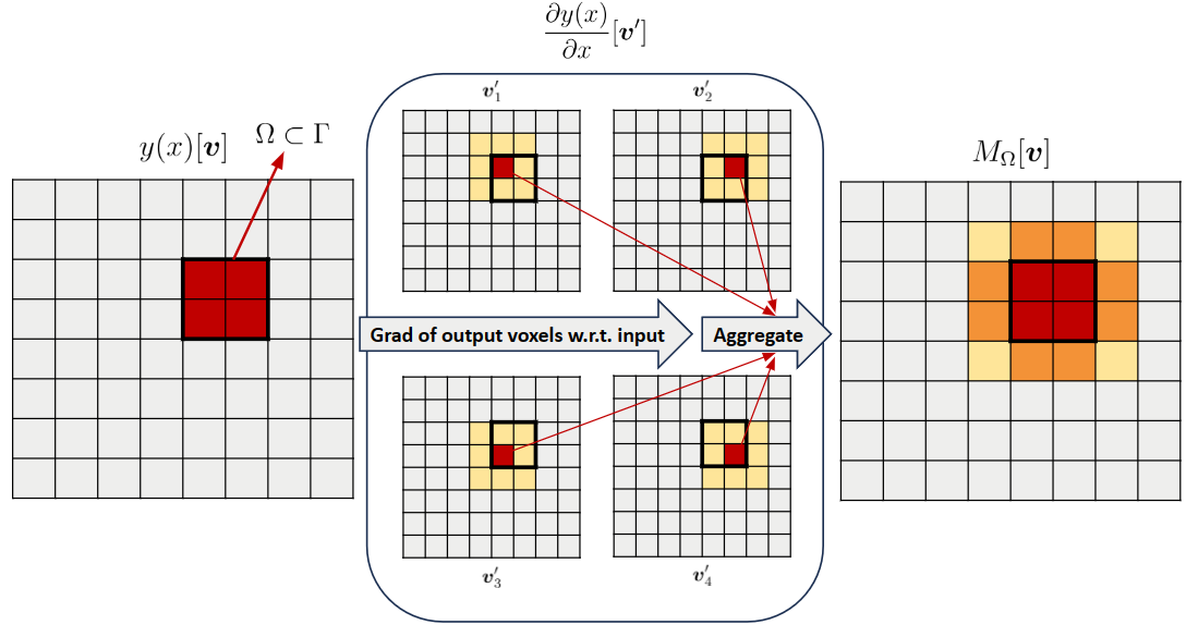
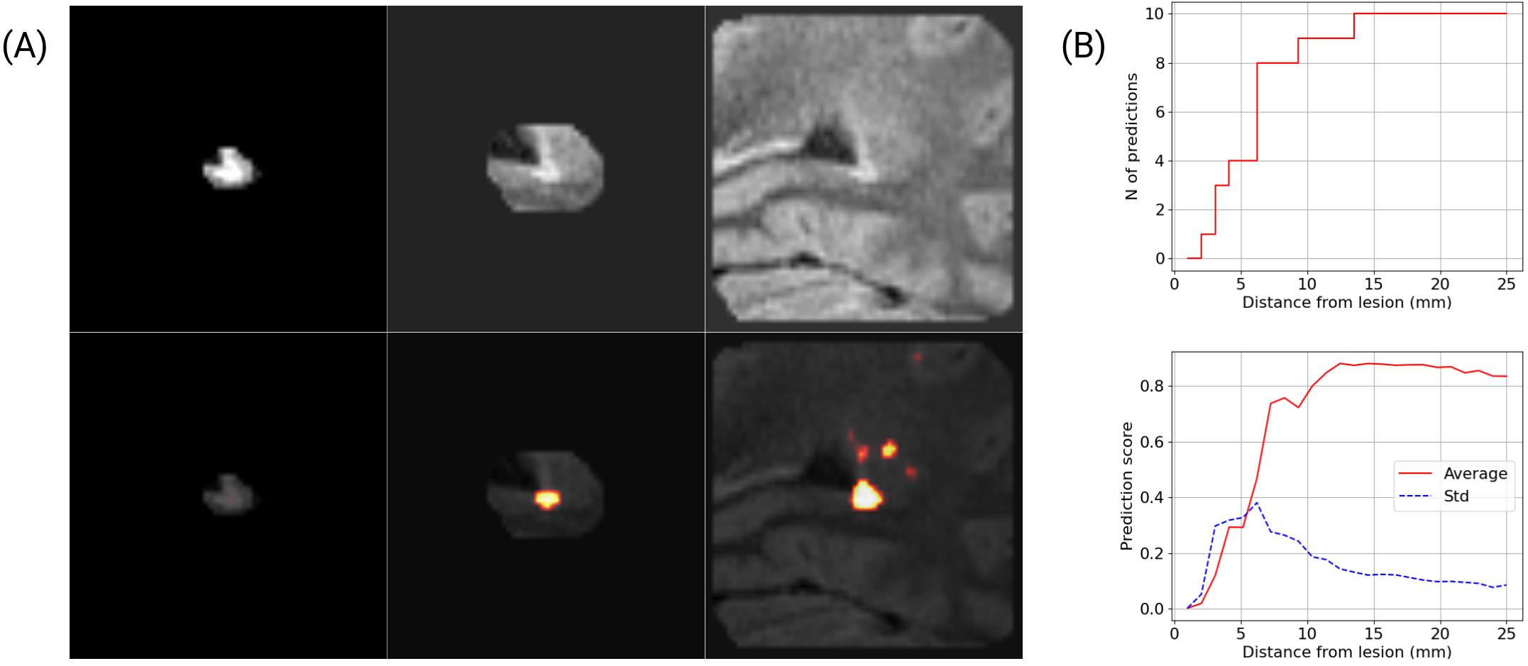
We trained and tested a 3D U-Net4 for white matter lesion (WML) segmentation on 687 MS patients, with fluid attenuated inversion recovery (FLAIR) and magnetisation prepared rapid gradient-echo (MPRAGE) scans collected at the University Hospital of Basel, Switzerland. We adopted the blob loss5 function to tackle instance imbalance in segmentation6. Ground truth (GT) lesion masks were annotated by three expert clinicians. Pre-processing steps included co-registration with the Elastix toolbox7,8, N4 bias correction9 and z-score normalization. True positive (TP) and false positive/negative (FP, FN) predictions were defined as connected components (connectivity of 2) having respectively a non-zero and zero overlap with GT. Binary lesion masks were obtained setting a threshold at 0.3 on predictions (lesion size > $$$5 mm^{3}$$$). We defined a discrete image10 as a three-dimensional function of the variable $$$\boldsymbol{v}=(v_1,... ,v_D)\in\mathbb{Z}^3$$$, taking values $$$x[\boldsymbol{v}]\in\mathbb{R}$$$, the image domain as $$$\Gamma\subset\mathbb{Z}^3$$$, the lesion domain $$$\Omega$$$ as a subset of $$$\Gamma$$$ with cardinality $$$|\Omega|$$$, and the output logits $$$y\left(x\right) [\boldsymbol{v}] \in \mathbb{R}$$$ as a map with the same dimensions as the input.We adapted SmoothGrad11 to address instance-level explanations by aggregating all saliency maps of voxels $$$\boldsymbol{v}'\in\Omega$$$. For a given lesion, the implementation consisted in: 1) injecting Gaussian noise $$$\mathcal{N}(0,\sigma)$$$ to obtain $$$N$$$ noisy versions of the input; 2) computing all saliency maps corresponding to voxels $$$\boldsymbol{v}'\in\Omega$$$ and determining their voxel-wise maximum (Fig.1); 4) combining $$$N=50$$$ noisy versions to obtain a lesion-level saliency map $$$M_\Omega\in\mathbb{R}$$$ (Eq.1):$$M_{\Omega}[\boldsymbol{v}] = \frac{1}{N} \sum_{n=1}^{N}\max_{\boldsymbol{v}'\in\Omega} \left[\frac{\partial y(x_{n})[\boldsymbol{v}']}{\partial x_{n}[\boldsymbol{v}]}\right].$$In a batch of 10 patients, we qualitatively evaluated the proposed saliency maps on 342 MS lesions, healthy tissue and additional synthetized lesions to understand their level of specificity in segmenting WML. Then, the relationship between the amount of perilesional tissue seen by the network and the prediction score was analyzed by: 1) masking out the input image with a mask that originally contains only the lesion 2) gradually applying morphological 3D dilation to include more surrounding voxels, to a maximum of $$$25 mm$$$ distance from the lesion's edges. At each iteration we observed the average and standard deviation across patients of the mean prediction score in $$$\Omega$$$, and the number of segmented lesions.
Results
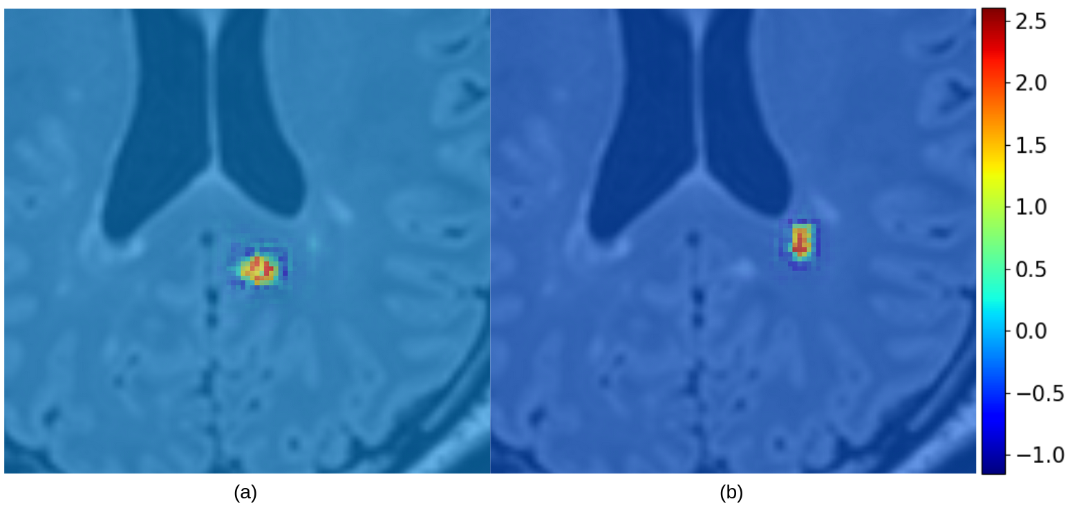
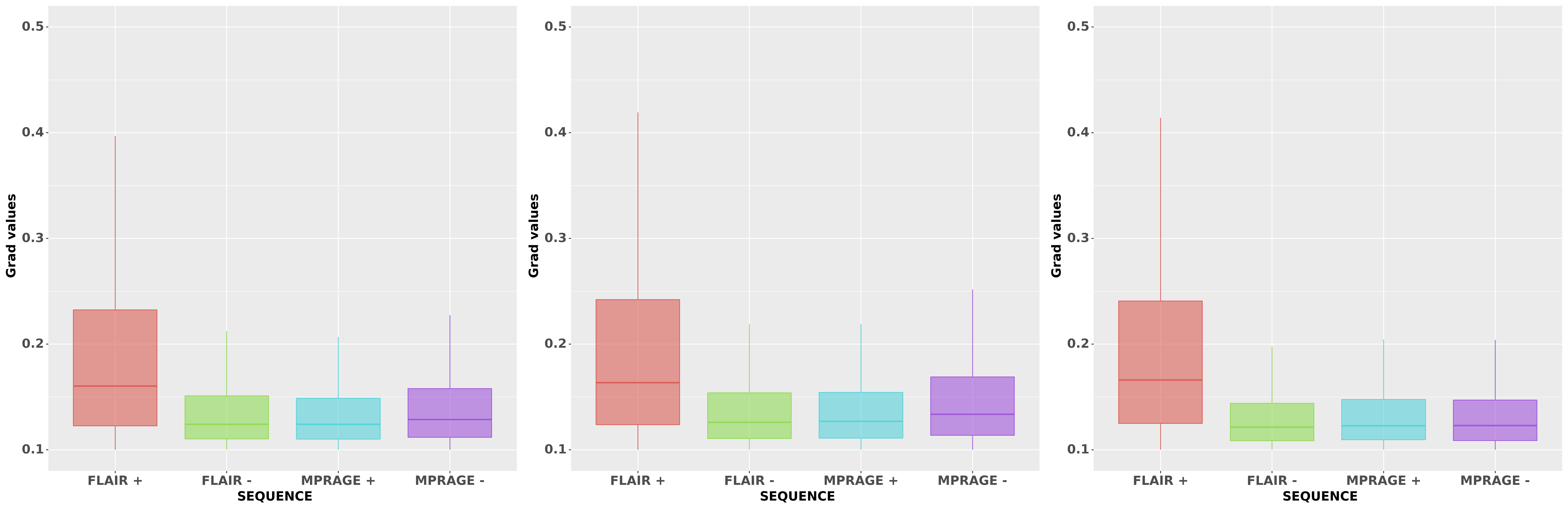
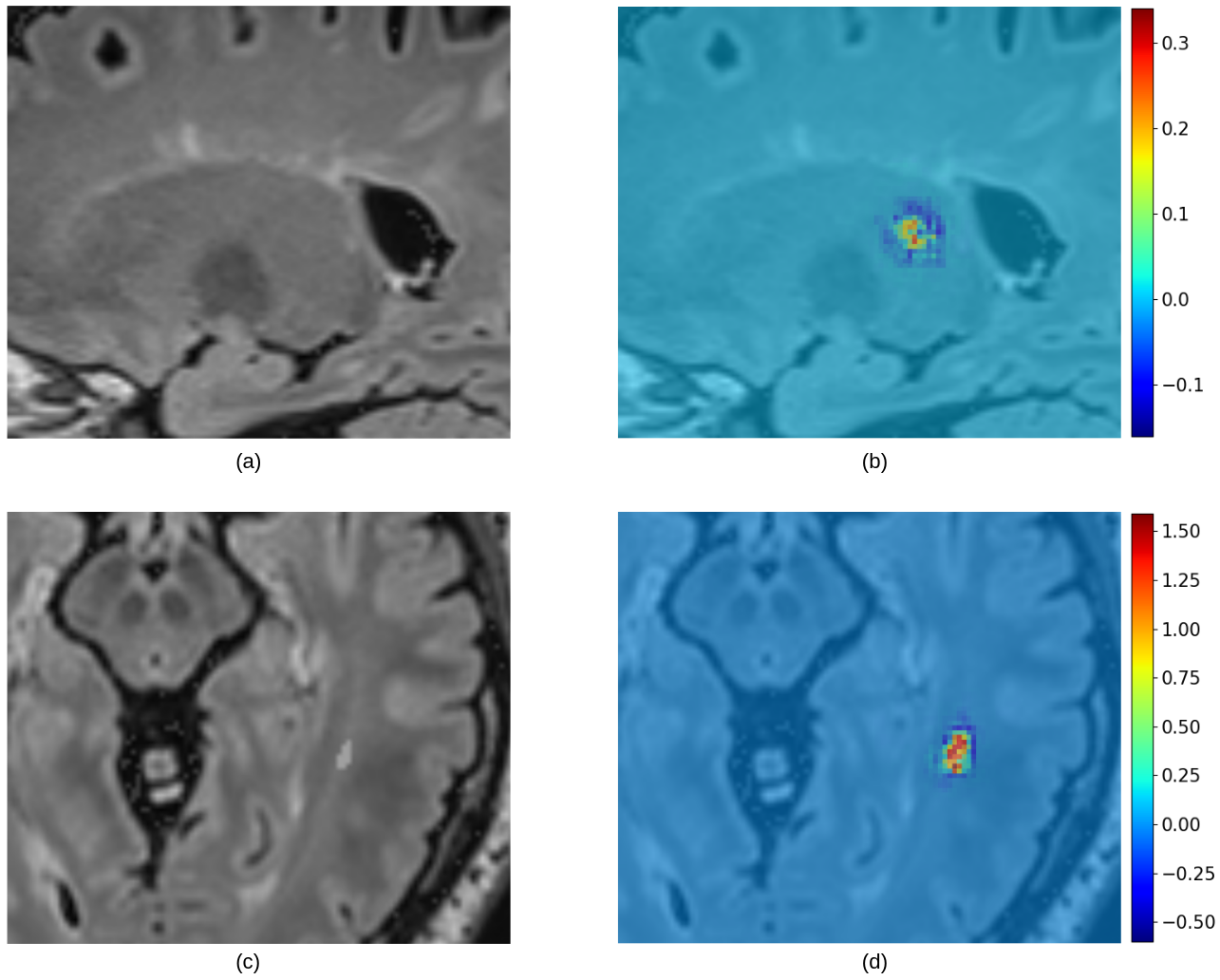
In saliency maps generated with respect to FLAIR, positive gradient values accumulate inside $$$\Omega$$$, while negative values populate the perilesional volume. For the MPRAGE, we observe a dual trend with negative values in $$$\Omega$$$. Voxels outside $$$\Omega$$$'s neighborhood present values close to zero, even when other lesions are in the proximity (Fig.2). The absolute values of saliency maps computed for FLAIR are consistently higher than for MPRAGE (Fig.3). Saliency maps generated from a volume with healthy tissue present gradient values with orders of magnitude that are 10-30 times smaller than values obtained for a lesion (Fig.4). However, scores and saliency maps obtained for synthetic lesions in the white matter are similar to the TP cases (Fig.4). The experiment on contextual information (Fig.5) shows that the prediction score for a lesion increases and plateaus after including perilesional tissue distant $$$12-15mm$$$ from the lesion border.Discussion
Thanks to the maximum operation in Eq.1, the absolute gradient values can be used to assess saliency across lesions and patients. The U-Net focuses more on FLAIR, compared to MPRAGE, during inference. This, along with experiments on synthetic lesions suggest that the network’s predictions rely predominantly on voxel intensities in FLAIR. However, a stable prediction was related to the amount of contextual information (i.e. healthy brain) from the perilesional volume.Conclusion
We proposed a method to provide instance-level explanations in semantic segmentation tasks. The study revealed fundamental insights in the decision process of a deep learning MS lesion segmentation network.Acknowledgements
This work was supported by the Hasler Foundation with the project MSxplain number 21042.References
1. Saranya, A., Subhashini, R. (2023). A systematic review of Explainable Artificial Intelligence models and applications: Recent developments and future trends. Decision Analytics Journal. 7. 100230. 10.1016/j.dajour.2023.100230.
2. Vinogradova, K., Dibrov, A., Myers, G. (2020). Towards Interpretable Semantic Segmentation via Gradient-weighted Class Activation Mapping. arXiv.
3 Sacha, M., Rymarczyk, D., Struski, Ł., Tabor, J., Zeliński, B. (2023). ProtoSeg: Interpretable Semantic Segmentation with Prototypical Parts. 10.48550/arXiv.2301.12276.
4. Çiçek, O., Abdulkadir, A., Lienkamp, S. S., Brox, T., and Ronneberger, O. (2016). 3D U-Net: Learning Dense Volumetric Segmentation from Sparse Annotation. arXiv.
5. Kofler, F., Shit, S., Ezhov, I., Fidon, L., Horvath, I., Al-Maskari, R., Li, H., Bhatia, H., Loehr, T., Piraud, M., Erturk, A., Kirschke, J., Peeken, J., Vercauteren, T., Zimmer, C., Wiestler, B., and Menze, B. (2022). Blob loss: instance imbalance aware loss functions for semantic segmentation. arXiv.
6. Malinin, A., Athanasopoulos, A., Barakovic, M., Cuadra, M. B., Gales, M. J. F., Granziera, C., Graziani, M., Kartashev, N., Kyriakopoulos, K., Lu, P.-J., Molchanova, N., Nikitakis, A., Raina, V., La Rosa, F., Sivena, E., Tsarsitalidis, V., Tsompopoulou, E., and Volf, E. (2022). Shifts 2.0: Extending The Dataset of Real Distributional Shifts. arXiv.
7. Klein, S., Staring, M., Murphy, K., Viergever, M., and Pluim, J. (2009). Elastix: A Toolbox for Intensity-Based Medical Image Registration. IEEE transactions on medical imaging, 29:196–205.
8. Shamonin, D., Bron, E., Lelieveldt, B., Smits, M., Klein, S., and Staring, M. (2014). Fast Parallel Image Registration on CPU and GPU for Diagnostic Classification of Alzheimer’s Disease. Frontiers in neuroinformatics, 7:50.
9. Tustison, N., Avants, B., Cook, P., Zheng, Y., Egan, A., Yushkevich, P., Gee, J. (2010). N4ITK: improved N3 bias correction. Medical Imaging, IEEE Transactions on. 29. 1310 - 1320. 10.1109/TMI.2010.2046908.
10. Depeursinge, A., Andrearczyk, V., Whybra, P., van Griethuysen, J., Müller, H., Schaer, R., Vallières, M., and Zwanenburg, A. (2020). Standardised convolutional filtering for radiomics. arXiv.
11. Smilkov, D., Thorat, N., Kim, B., Viégas, F., and Wattenberg, M. (2017). SmoothGrad: removing noise by adding noise. CoRR.
Figures