2224
Understanding the Trustworthiness of Saliency Maps for Biomarker Research in 3D Medical Imaging Classification1School of Computer Science, University of Sydney, Sydney, Australia, 2Brain and Mind Centre, University of Sydney, Sydney, Australia
Synopsis
Keywords: Analysis/Processing, Machine Learning/Artificial Intelligence, saliency maps; biomarkers
Motivation: It is significant to understand if saliency maps can be considered as potential biomarkers by providing reliable anatomical information in 3D medical imaging classification.
Goal(s): We found saliency maps can provide different (even mutually exclusive) information with randomised models. It is necessary to estimate the robustness of saliency maps under the stochastic training process.
Approach: We introduced a novel method by re-organising the saliency scores in the saliency maps and quantify the inter-map difference for estimating the robustness of saliency maps.
Results: All selected explanation methods were not able to exhibit strong performance in the estimation of robustness of saliency maps.
Impact: Our estimation provides evidence that saliency maps are not competent to maintain the robustness under the stochastic training process. Researchers should be critically careful when utilising saliency maps as biomarkers for interpretation.
Introduction
Convolutional neural networks (CNNs) have become the de facto state-of-the-art algorithm for the classification of 3D medical images1. Their ability to encode local and long-term relationships between voxels and regions in the image could help uncover unknown biomarkers and provide an early diagnosis to improve patient treatment and prognosis. However, as CNNs grows in complexity and impact, their decision mechanisms are considered inconceivable as a“ black box”. Researchers has been committed to revealing the inner working pattern of CNNs with explanation methods. Typically, in the medical imaging analysis field, it is accomplished by saliency maps2, which demonstrate the visualised interpretation by representing saliency scores related with their contribution to the network outputs. To investigate the potential of saliency maps as biomarkers for 3D medical imaging classification, we believe that it is important to conduct quantitative analysis for estimating the robustness of saliency maps.Methodology
Dataset In this study, we used the publicly available OASIS-3 neuroimaging dataset3 for training CNNs and producing saliency maps. The subjects in the dataset were divided in two group depending on their diagnosis – 166 subjects in the condition of Alzheimer’s disease (AD) and 512 subjects in the condition of Health control (HC). All images were pre-processed by the fmriprep toolbox4, including bias correction and registration to the MNI space.Network Architecture In this study, we defined the network architecture containing 5 convolutional blocks and 1 fully connected (FC) layer. The convolutional block was composed of a 3D convolutional layer, a 3D batch normalisation layer and a RELU activation layer. Additionally, a following max-pooling layer (set scale to 2) was applied after each convolutional block.
Explanation method In this study, we introduced six common explanation methods including LayerGradCAM5, Guided Backpropagation6, Deconvolution7, Guided GradCAM5, Gradient SHAP8 and Input X Gradient9.
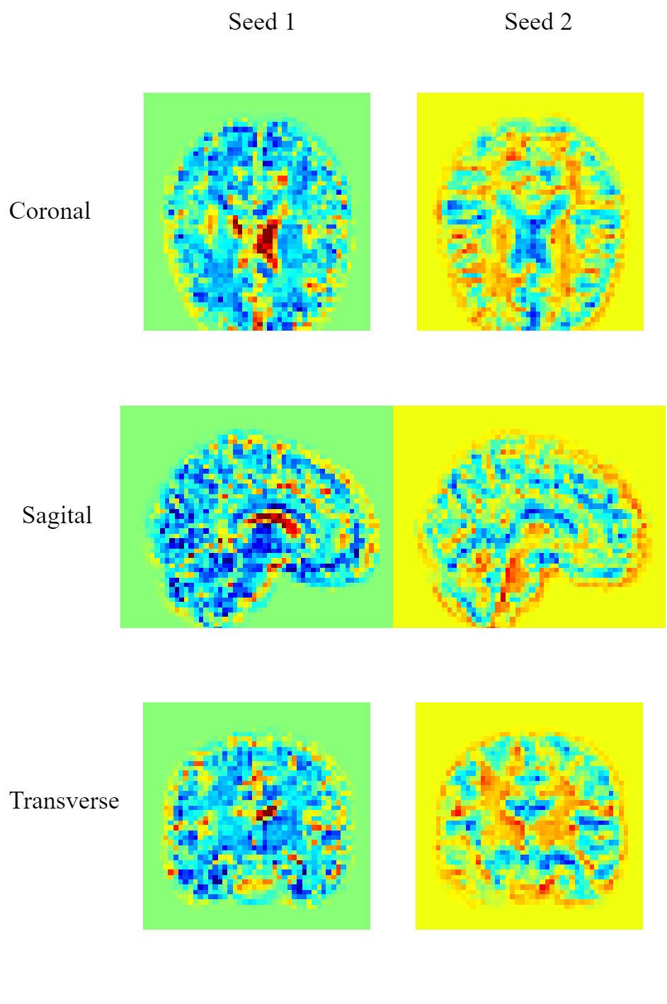
Homogeneity An ideal saliency map, from the perspective of utility of biomarkers, would have perfect recall (finding all regions of interest) without labelling any voxels outside the regions of interest as positive (perfect precision) under the stochastic training process. However, we noticed that saliency maps could even provide mutually exclusive information from an explanation method. As shown in Figure. 1, the same CRF area in two saliency maps generated by randomized models were granted to positive (region of interest) and negative (region of non-interest) saliency scores. In the case, we cannot directly compare the inter-map difference as the evidence of saliency maps’ consistency since it could be caused by the model – in essence, saliency maps correctly express what the model learned while models in the stochastic training process learned different features.
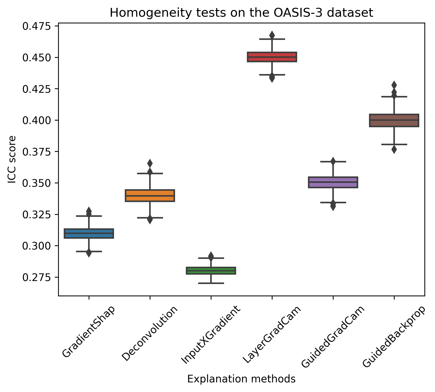
To solve the issue, we employed an estimation method named saliency attention. To be specific, given a saliency map produced by an explanation method, we collected the saliency scores in the map to an array. Afterwards, we ranked the array in the descending order and recorded the representation of the relative position of each saliency score. The saliency scores in the same position of each saliency map generated by randomized models were assembled to a group. Then we conducted the customized Intra-class Correlation Coefficient (ICC)10 measurement to each group for quantifying the homogeneity of saliency maps in the stochastic training process, where models were identified as raters and the ICC reliability scores were computed based on each group.
Experimental Results and Discussion
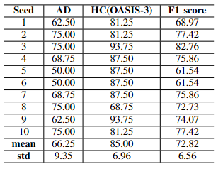
We implemented a 10-random-seed experiment to statistically estimate the robustness of saliency maps. The overall accuracy was 0.75 among 10 models and the accuracy of AD was much lower than HC, suggesting that the network could cope with the heavy imbalance of the dataset (See Fig. 2 for the details of testing results). As shown in Fig. 3, all selected explanation methods failed to achieve more than 0.5 ICC score, indicating that their saliency maps were not able to maintain the robustness – to clarify, given the saliency maps generated by 10 randomised trained models, if a region was allocated high positive saliency scores in a saliency map, there was likely not a region which was rendered similar scores correspondingly in another saliency map.Conclusion
In this study, we evaluated popular saliency maps for CNNs trained stochastically on the OASIS-3 datasets in terms of a key criteria for the trustworthiness as biomarkers. Our proposed method was component to effectively reduce the influence of external interference factors, such as saliency maps correctly reflected what the model learned while randomised models learned different features. According to our experiment's results, researchers should be critically careful when utilising saliency maps as biomarkers for anatomical interpretation and disease cognition.Acknowledgements
I would like to express our sincere gratitude to the individuals and organizations that have supported and contributed to the success of this research project.
First and foremost, I am deeply appreciative of my supervisors, Associate Professor Weidong Cai, Dr. Chenyu Wang, Dr. Mariano Cabezas and Dr. DongnanLiu for their invaluable guidance, expertise, and unwavering support throughout the duration of this study. Their mentorship and constructive feedback have been instrumental in shaping the direction and quality of my work.
We would also like to thank Sydney Neuroimaging Analysis Centre, for their assistance in providing access to essential equipment and facilities. This research would not have been possible without their generous help.
This research work was a collective effort, and I am thankful to everyone who played a role, however small, in its successful completion.
References
1. M. Jamshidi, A. Lalbakhsh, J. Talla, Z. Peroutka, F. Hadjilooei, P. Lal-bakhsh, M. Jamshidi, L. La Spada, M. Mirmozafari, M. Dehghaniet al., “Artificial intelligence and covid-19: deep learning approachesfor diagnosis and treatment,” Ieee Access, vol. 8, pp. 109 581–109 595,2020.
2. M. S. Ayhan, L. B. K ̈ummerle, L. K ̈uhlewein, W. Inhoffen, G. Aliyeva,F. Ziemssen, and P. Berens, “Clinical validation of saliency maps forunderstanding deep neural networks in ophthalmology,” Medical ImageAnalysis, vol. 77, p. 102364, 2022.
3. P. J. LaMontagne, T. L. Benzinger, J. C. Morris, S. Keefe, R. Hornbeck,C. Xiong, E. Grant, J. Hassenstab, K. Moulder, A. G. Vlassenko et al.,“Oasis-3: longitudinal neuroimaging, clinical, and cognitive dataset fornormal aging and alzheimer disease,” MedRxiv, pp. 2019–12, 2019.
4. O. Esteban, C. J. Markiewicz, R. W. Blair, C. A. Moodie, A. I. Isik,A. Erramuzpe, J. D. Kent, M. Goncalves, E. DuPre, M. Snyder et al.,“fmriprep: a robust preprocessing pipeline for functional mri,” Naturemethods, vol. 16, no. 1, pp. 111–116, 2019.
5. R. R. Selvaraju, M. Cogswell, A. Das, R. Vedantam, D. Parikh, andD. Batra, “Grad-cam: Visual explanations from deep networks viagradient-based localization,” in Proceedings of the IEEE internationalconference on computer vision, 2017, pp. 618–626.
6. J. T. Springenberg, A. Dosovitskiy, T. Brox, and M. Riedmiller,“Striving for simplicity: The all convolutional net,” arXiv preprintarXiv:1412.6806, 2014.
7. M. D. Zeiler and R. Fergus, “Visualizing and understanding convo-lutional networks,” in Computer Vision–ECCV 2014: 13th EuropeanConference, Zurich, Switzerland, September 6-12, 2014, Proceedings,Part I 13. Springer, 2014, pp. 818–833.
8. S. M. Lundberg and S.-I. Lee, “A unified approach to interpretingmodel predictions,” in Advances in Neural Information ProcessingSystems, I. Guyon, U. V. Luxburg, S. Bengio, H. Wallach, R. Fergus,S. Vishwanathan, and R. Garnett, Eds., vol. 30. Curran Associates,Inc., 2017.
9. A. Shrikumar, P. Greenside, A. Shcherbina, and A. Kundaje, “Not justa black box: Learning important features through propagating activationdifferences,” arXiv preprint arXiv:1605.01713, 2016.
10. J. P. Weir, “Quantifying test-retest reliability using the intraclass corre-lation coefficient and the sem,” The Journal of Strength & ConditioningResearch, vol. 19, no. 1, pp. 231–240, 2005.
Figures