2006
Renal perfusion quantification using multi delay Pseudo-continuous Arterial Spin Labeling: Comparison of results at 1.5T and 3T field strengths1Department of Radiology, Clínica Universidad de Navarra, Pamplona, Navarra, Spain, 2Instituto de Investigación Sanitaria de Navarra, IDISNA, Pamplona, Navarra, Spain, 3Department of Nephrology, Clínica Universidad de Navarra, Pamplona, Navarra, Spain, 4Siemens Healthcare, Madrid, Spain
Synopsis
Keywords: Arterial Spin Labelling, Perfusion, T1 mappinng
Motivation: Pseudo-continuous Arterial Spin Labeling (PCASL) MRI is a promising technique for assessing renal perfusion. Previous studies have been carried out at 1.5T and 3T field strengths, but a comparison of data acquired at both field strengths has never been performed.
Goal(s): The aim of this work was to assess the effects of field strength on the measured perfusion signal and to evaluate the reproducibility of renal PCASL at both fields
Approach: Healthy volunteers underwent repeated scans on both scanners, spaced a week apart.
Results: The results showed excellent reproducibility and minimal differences in RBF, ATT and T1 values between visits and field strengths.
Impact: The similarity in the study results across both field strengths underscore the potential for expanding PCASL-based renal perfusion assessment, increasing the technique accessibility, and widening diagnostic capabilities.
INTRODUCTION
Arterial Spin Labeling (ASL) is a promising technique for renal perfusion assessment. Different imaging techniques at independent magnetic filed strengths (1.5T and 3T) have been used to assess renal perfusion1. However, there is a notable absence of comparative research at both field strengths. Therefore, this study aims to compare the outcomes and reproducibility of renal ASL at both 1.5T and 3T. These findings might contribute to ASL reliability in assessing renal perfusion, supporting its potential integration into clinical practice.METHODS
Subjects and Study Design:Written informed consent was obtained from subjects. Urine and blood were obtained to measure the estimated glomerular filtration rate (eGFR) with the CKD-EPI equation2. Eight healthy volunteers (eGFR>90ml/min/1.73m2, mean age±standard deviation (SD)=32±7.9 years) were scanned twice within the same day on 1.5T Aera and 3T Skyra MRI scanners (Siemens Healthcare), using 18-channel body and spine coils. The same protocol was repeated with a median of seven days (range=1-17 days).
MRI Protocol:
Pseudo-continuous ASL (PCASL) sequence employing six different post-labeling delays (PLDs), with background suppression (BS) and SE-EPI readout. Pre-saturation pulses were applied before the labeling pulses. BS was achieved using a slice-selective FOCI pulse before labeling and two non-selective tangent/hyperbolic tangent pulses after labeling. Pulse timings were optimized for each PLD to suppress static tissue signal to 15%. This optimization was performed for each field strength considering the expected kidney T1 values. PCASL were acquired with and without BS pulses for the PLD=1.3s, to estimate the efficiency of the BS pulses.
T1 Inversion Recovery sequence employing 16 inversion times and SE-EPI readout. Other sequence parameters are described in Table 1.
Image processing:
All the images underwent registration in Elastix3 using a groupwise registration method. Subsequent analysis was conducted using custom scripts in Matlab (Mathworks). T1 maps were generated by fitting the signal to the inversion-recovery equation [1]:
$$S_k=M_0(1-2e^{-TI_k/T1)}+M_0e^{-TR/T1})$$
To compute Renal Blood Flow (RBF) and Arterial Transit Time (ATT) maps, a voxel-by-voxel approach was employed, fitting the data to the one-compartment Buxton4 model, with the assumption that by the time of image acquisition, labeled spins remained in the blood [2]:
$$(SI_C-SI_L)_t=\begin{cases}0&\text{if }0<\tau_t+\text{PLD}_t<\text{ATT}\\\frac{2\alpha\text{T1}_b}{6000\lambda}M_0RBFe^{-\frac{\text{ATT}_t}{\text{T1}_b}}(1-e^{-\frac{(\tau_t+\text{PLD}_t-\text{ATT})}{\text{T1}_b}})&\text{if }\text{ATT}<\tau_t+\text{PLD}_t<\tau_t+\text{ATT}\\\frac{2\alpha\text{T1}_b}{6000\lambda}M_0RBFe^{-\frac{\text{PLD}_t}{\text{T1}_b}}(1-e^{-\frac{\tau_t}{\text{T1}_b}})&\text{if } \tau_t+\text{ATT}<\tau_t+\text{PLD}_t \end{cases}$$
where $$$(SI_C - SI_L)$$$ is the signal difference between control and label images for each PLD, $$$\alpha=0.75\times0.9\times0.9$$$ is the labeling efficiency, considering PCASL efficiency and the effects of 2 BS pulses, $$$\lambda=0.9$$$mL/g is the tissue-blood partition coefficient, $$${T1_{b}}=1.48$$$s and $$$1.65$$$s are the longitudinal relaxation times of blood at 1.5T and 3T, respectively and $$$\tau$$$ is the labelling duration. Regions of Interest (ROIs) in the cortex and medulla were manually drawn in the T1 maps and used to obtain mean values by averaging both kidneys.
Statistical analysis:
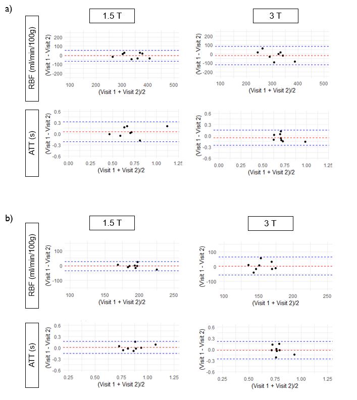
Differences between field strengths, were tested by paired t-test. Reproducibility was assessed by Bland-Altman plots and by the inter-session within subject coefficient of variation (wsCV), calculated as the root mean square of the squared ratio of the SD to the mean for each subject of the two repeated measurements5.
RESULTS AND DISCUSSION
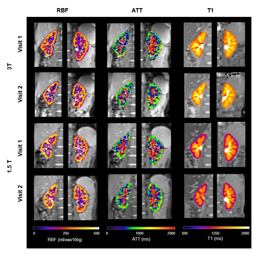
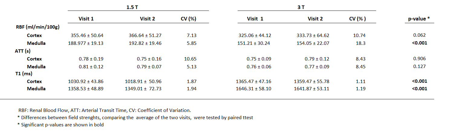
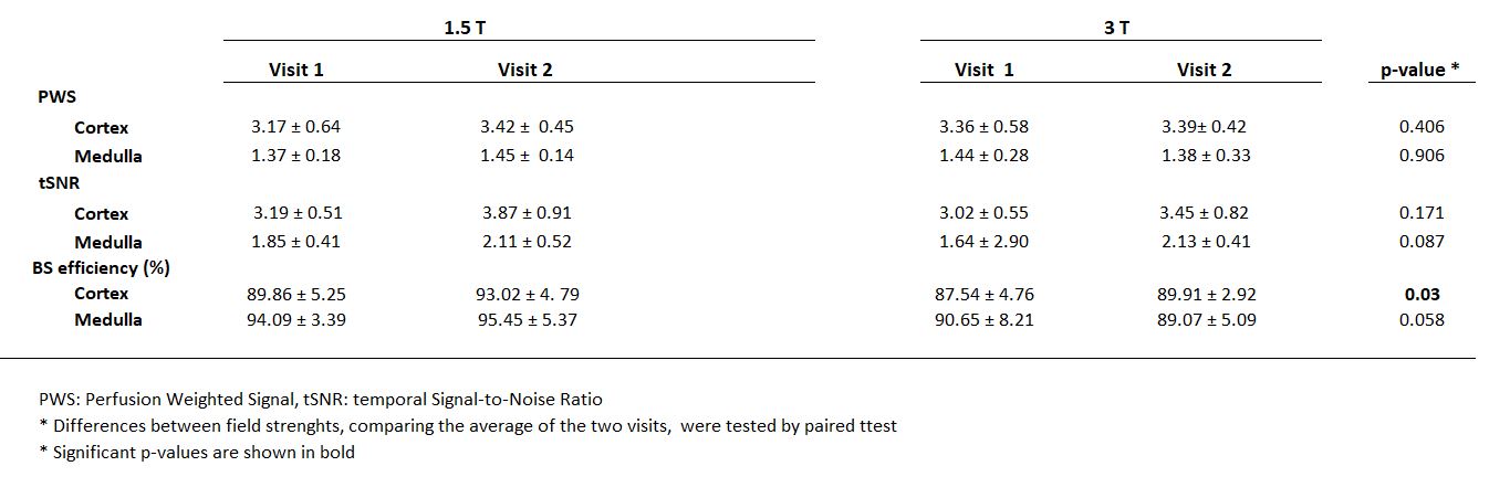
RBF, ATT, and T1 maps for a representative subject are depicted in Figure 1.Table 2 provides averaged cortical and medullary values across the group, for each visit and field strength. T1 measurements aligned with literature values6, and as expected, T1 values were longer at 3T compared to 1.5T. Inter-session wsCVs for T1 in the cortex and medulla were low, indicating excellent reproducibility (<2% for 1.5T and <1.2% for 3T). RBF and ATT measurements obtained during both visits and at both field strengths yielded remarkably similar results, consistent with the literature1,6-7, with no statistically significant differences between field strengths, except for the RBF values in the medulla (p<0.001), which were higher at 1.5T. It is worth noting that cortical RBF values were also 10% higher at 1.5T (although the differences did not reach statistical significance). These data were also reproducible, with cortical and medullary wsCVs<11% for RBF and ATT at both 1.5T and 3T, except for the medulla at 3T (wsCV=18.3%). Bland-Altman plots (Figure 2) showed good reproducibility between visits for both the cortex and medulla. Perfusion weighted signal (PWS), temporal Signal-to-Noise Ratio (tSNR), and BS efficiency for PLD=1.3s were also obtained (Table 3). Results showed a higher BS efficiency in the 1.5T scans, which could be attributed to a more uniform magnetic field, which partly explain the observed differences in RBF, that could also be due to a higher labeling efficiency, at 1.5T compared to 3T. Although this parameter was not measured.CONCLUSION
Similarity in results across both field strengths highlights the potential for wider adoption of PCASL-based renal perfusion assessment and support its use in multicenter clinical studies.Acknowledgements
Leyre Garcia-Ruiz received PhD grant support from Asociación de Amigos de la Universidad de Navarra. This project was supported by the Government of Navarra under the frame of ERA PerMed (ERAPERMED2020-326 - RESPECT) and under grant: PC181-182 RM-RENAL.
References
1. Odudu A, Nery F, Harteveld AA, Evans RG, Pendse D, Buchanan CE, Francis ST, Fernández-Seara MA. Arterial spin labelling MRI to measure renal perfusion: a systematic review and statement paper. Nephrol Dial Transplant. 2018 Sep 1;33(suppl_2):ii15-ii21. doi: 10.1093/ndt/gfy180.
2. Levey AS, Stevens LA, Schmid CH, Zhang YL, Castro AF 3rd, Feldman HI, Kusek JW, Eggers P, Van Lente F, Greene T, Coresh J; CKD-EPI (Chronic Kidney Disease Epidemiology Collaboration). A new equation to estimate glomerular filtration rate. Ann Intern Med. 2009 May 5;150(9):604-12. doi: 10.7326/0003-4819-150-9-200905050-00006.
3. Klein S, Staring M, Murphy K, Viergever MA, Pluim JPW: elastix: A Toolbox for Intensity-Based Medical Image Registration. IEEE Trans Med Imaging 2010; 29:196–205.
4. Buxton RB, Frank LR, Wong EC, Siewert B, Warach S, Edelman RR. A general kinetic model for quantitative perfusion imaging with arterial spin labeling. Magn Reson Med. 1998 Sep;40(3):383-96. doi: 10.1002/mrm.1910400308.
5. Bland JM, Altman DG. Measurement error. BMJ. 1996 Sep 21;313(7059):744.
6. Cox EF, Buchanan CE, Bradley CR, Prestwich B, Mahmoud H, Taal M, Selby NM, Francis ST. Multiparametric Renal Magnetic Resonance Imaging: Validation, Interventions, and Alterations in Chronic Kidney Disease. Front Physiol. 2017 Sep 14;8:696. doi: 10.3389/fphys.2017.00696.
7. Kim DW, Shim WH, Yoon SK, Oh JY, Kim JK, Jung H, Matsuda T, Kim D. Measurement of arterial transit time and renal blood flow using pseudocontinuous ASL MRI with multiple post-labeling delays: Feasibility, reproducibility, and variation. J Magn Reson Imaging. 2017 Sep;46(3):813-819. doi: 10.1002/jmri.25634.
Figures
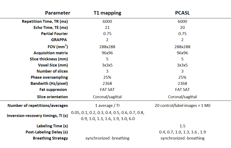
Table 1: Description of T1 mapping and Pseudo Continuous Arterial Spin labeling sequences parameters employed in the MRI protocol. Other PCASL parameters: unbalanced, B1 average = 1.6µT, average gradient = 0.5mT/m and ratio Gmax/Gave = 7.