1978
4D Flow MRI Velocity Enhancement and Anti-Aliasing Using Divergence Free Potential in Neural Networks1Biomedical Imaging Center, Pontificia Universidad Catolica de Chile, Santiago, Chile, 2Millennium Institute for Intelligent Healthcare Engineering, iHEALTH, Santiago, Chile, 3Department of Electrical Engineering, Pontificia Universidad Catolica de Chile, Santiago, Chile, 4Departamento de Informática, Universidad Técnica Federico Santa Maria, Santiago, Chile, 5School of Electrical Engineering, Pontificia Universidad Catolica de Valparaíso, Valparaíso, Chile, 64Department of Mechanical Engineering, Universidad Técnica Federico Santa Maria, Santiago, Chile, 7Faculty of Engineering, Universidad Alberto Hurtado, Santiago, Chile, 8Department of Medical Imaging and Radiation Sciences, Monash University, Melbourne, Australia
Synopsis
Keywords: Analysis/Processing, Velocity & Flow, Velocity enhancement, Anti-aliasing
Motivation: 4D flow MRI suffers from different sources of noise and aliasing artifacts. However, the existing techniques for enhancing velocities in 4D flow MRI encounter reliability problems with varying flow patterns or acquisition parameters.
Goal(s): Our goal was to develop a velocity enhancement an anti-aliasing technique for 4D Flow MRI that can be easily applied to diverse flow types.
Approach: We incorporate a vector potential into a neural network to predict velocity fields that strictly adhere to the divergence-free condition.
Results: Results from simulated 4D flow MRI images demonstrate significant noise reduction and aliasing correction.
Impact: The proposed Physics-Informed Neural Network enables the recovery of noise-free and aliasing artifact-free velocity fields using divergence-free terms in the network without the need for tuning hyperparameters in the training function, enhancing the applicability of these networks to different datasets.
Introduction
4D flow MRI allows the quantification of advanced hemodynamic parameters that provide valuable information to characterize cardiovascular diseases. However, 4D flow technique suffers from random acquisition noise, low spatial and temporal resolution, velocity aliasing and respiratory motion1 . To improve the accuracy of flow imaging, 4D flow MRI data can be constrained according to physical principles. For instance, by considering blood as an incompressible fluid, a divergence free constraint could be used to enhance velocity measurements. Current methods for optimizing divergence-free 4D flow MRI suffer from reliability issues when applied to different flow types or modified acquisition parameters. Regularized optimization techniques2,3,4 balance data consistency and divergence-free conditions but lack guaranteed optimal weighting parameters, influenced by data quality. Projection-based methods5,6 vary depending on chosen bases and filtering procedures, limiting their applicability across diverse flow types. While deep learning techniques, such as 4DFlowNet7 and physics-informed neural networks8 show promise, 4DFlowNet is restricted to specific conditions and may not handle pathological flow patterns, and physics-informed networks require tuning of hyperparameters with no guarantee of physics compliance due to a lack of inductive bias in the model. In this work, we include a vector potential formulation9 as an inductive bias of a neural network to only predict velocity fields that are strictly divergence free. Therefore, the network predicts the best-fitting divergence-free velocity field for the data, without having to balance the physics regularization.Methods
For 3D incompressible flows, a divergence-free vector potential9 is introduced such that:$$\vec{V}=\nabla \times \Phi=\left(\frac{\partial \Phi_z}{\partial y}-\frac{\partial \Phi_y}{\partial z}, \frac{\partial \Phi_x}{\partial z}-\frac{\partial \Phi_z}{\partial x}, \frac{\partial \Phi_y}{\partial x}-\frac{\partial \Phi_x}{\partial y}\right)=(u, v, w) \qquad (1)$$
Thus, the velocity field $$$\vec{V}$$$ satisfies the continuity equation automatically,
$$ \nabla \cdot \vec{V}=\nabla \cdot(\nabla \times \vec{\Phi})=0 \qquad (2)$$
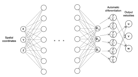
We use a fully connected neural network with the spatial coordinates as input and estimate a vector potential as defined in (1), rather than directly estimating the velocities. Instead, we compute the velocities with automatic differentiation (Figure 1). The loss function consists of the data fidelity term formulated by Fathi et al.8 to also address aliasing artifacts. This term considers the difference between the neural network estimated signal ($$$S_{NN}$$$) and the original signal ($$$S_{MR}$$$).
$$ \begin{gathered}L=\left\|S_{N N}-S_{M R}\right\|_2 \\S_{N N}=m_{M R} e^{-i 2 \pi \vec{u}_{N N}} \qquad (3)\\S_{M R}=m_{M R} e^{-i 2 \pi \vec{u}_{M R}}\end{gathered} $$
The algorithm was analyzed using computational fluid dynamics (CFD) simulations of a vascular model of an aorta[10] with one timeframe on peak systole. A 4D flow MRI image with parameters taken from11 (VENC of 210 cm/s and voxel size of 2.5 × 2.5 × 2.5 mm3), was generated evaluating the signal equation for gradient-echo sequence as:
$$ \left.S^a(k(t))=\int_B M_0\left(r_0\right) e^{-i \pi / V E N C v_a\left(r_0\right)} e^{-t / T_2^*\left(r_0\right)} e^{-i 2 \pi k(t)-r(t)} d r\right) . \qquad (4)$$
with $$$a = x,y,z$$$ and $$$v_a$$$ the fluid velocity. The k-space locations and timings were generated using realistic magnetic gradients. The motion of flowing spins was considered in Equation (4) using a first order Taylor expansion of $$$r(t)$$$.
We simulated aliasing artifacts and added complex gaussian noise to (15%, 20%, and 25% of maximum magnitude) the signals in training. The neural architecture consisted of 7 layers with 40 neurons each. We computed the root mean square velocity error (VRMSE) in cm/s and the directional error (DE)3 ($$$v_i^r$$$ is the reference velocity and $$$v_i^d$$$ the estimated velocity)
$$ V R M S E=\sqrt{\frac{1}{N} \sum_i\left|v_i^r-v_i^r\right|^2}, \quad D E=\frac{1}{N} \sum_i\left(1-\frac{\left|v_l^r \cdot v_i^d\right|}{\left|v_i^r\right|\left|v_i^d\right|}\right) \qquad (5)$$
Results
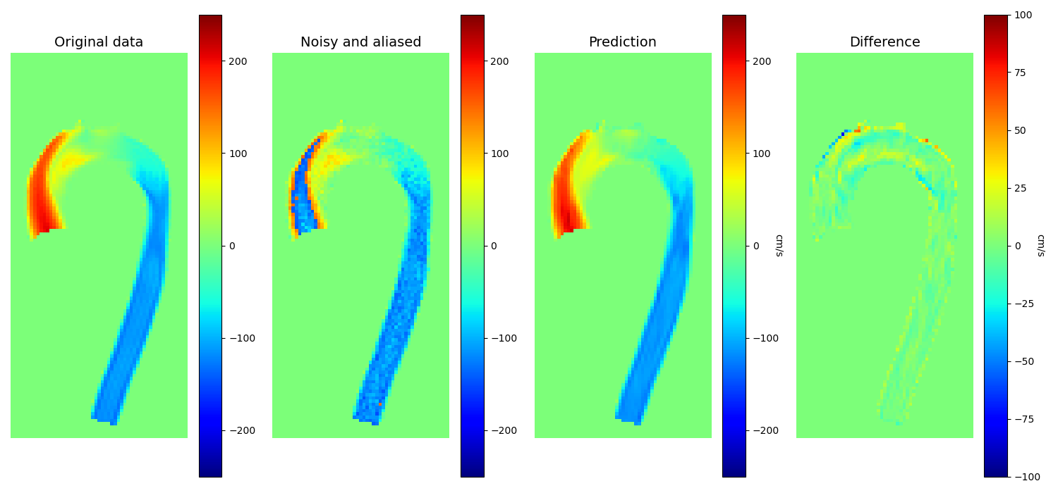
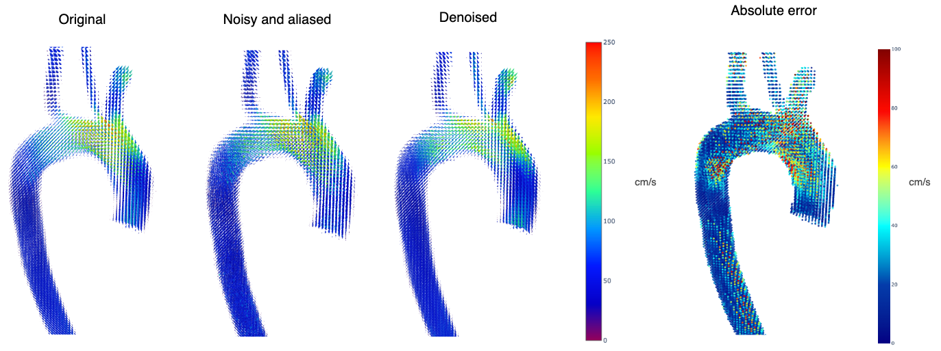
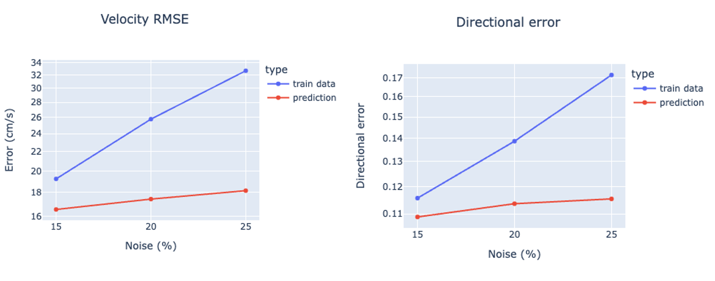
The algorithm demonstrated excellent performance, even in the presence of aliasing (Figure 2). The VNRMS and DE were both reduced at various noise levels (Figure 4). In Figure 2 and Figure 3, we observed larger errors between the corrected and original velocity values in the borders of the aorta and the best predictions were located near the centerline.Discussion
Our preliminary results shows that a neural network with divergence-free vector potential can successfully enhance 4D flow images with aliasing artifacts and noise. Furthermore, unlike previous techniques, we evaluate our algorithm with a 4D Flow MRI image generated from the signal equation of a gradient-echo sequence. Previous techniques only interpolate CFD velocities to a cartesian grid and then codify the velocities as complex MRI signals, leaving aside MRI acquisition factors such as temporal averaging or phase accumulation. Our results showed larger errors in the borders of the vessel. To reduce these errors, we will consider proper boundary conditions for a better velocity enhancement. We will also include the time dimension and experiment with real data to further validate the algorithm's effectiveness.Acknowledgements
This work was funded by ANID - Millennium Science Initiative Program - ICN2021_004. ANID-FONDECYT de iniciación en investigación 1120048, ANID-Fondecyt Postdoctorado #3220266 and ANID-Fondecyt 1231535.References
[1]P. Dyverfeldt et al., “4D flow cardiovascular magnetic resonance consensus statement,” J. Cardiovasc. Magn. Reson., vol. 17, no. 1, p. 72, Dec. 2015, doi: 10.1186/s12968-015-0174-5.
[2]E. Bostan, S. Lefkimmiatis, O. Vardoulis, N. Stergiopulos, and M. Unser, “Improved Variational Denoising of Flow Fields with Application to Phase-Contrast MRI Data,” IEEE Signal Process. Lett., vol. 22, no. 6, pp. 762–766, Jun. 2015, doi: 10.1109/LSP.2014.2369212.
[3]J. Mura et al., “Enhancing the Velocity Data From 4D Flow MR Images by Reducing its Divergence,” IEEE Trans. Med. Imaging, vol. 35, no. 10, pp. 2353–2364, Oct. 2016, doi: 10.1109/TMI.2016.2570010.
[4]J. Zhang et al., “Divergence-Free Constrained Phase Unwrapping and Denoising for 4D Flow MRI Using Weighted Least-Squares,” IEEE Trans. Med. Imaging, vol. 40, no. 12, pp. 3389–3399, Dec. 2021, doi: 10.1109/TMI.2021.3086331.
[5]E. Deriaz and V. Perrier, “Divergence-free and curl-free wavelets in two dimensions and three dimensions: application to turbulent flows,” J. Turbul., vol. 7, p. N3, Jan. 2006, doi: 10.1080/14685240500260547.
[6]F. Ong et al., “Robust 4D flow denoising using divergence-free wavelet transform: 4D Flow Denoising with DFW Transform,” Magn. Reson. Med., vol. 73, no. 2, pp. 828–842, Feb. 2015, doi: 10.1002/mrm.25176.
[7]E. Ferdian et al., “4DFlowNet: Super-Resolution 4D Flow MRI Using Deep Learning and Computational Fluid Dynamics,” Front. Phys., vol. 8, p. 138, May 2020, doi: 10.3389/fphy.2020.00138.
[8]M. F. Fathi et al., “Super-resolution and denoising of 4D-Flow MRI using physics-Informed deep neural nets,” Comput. Methods Programs Biomed., vol. 197, p. 105729, Dec. 2020, doi: 10.1016/j.cmpb.2020.105729.
[9]G. J. Hirasaki and J. D. Hellums, “A general formulation of the boundary conditions on the vector potential in three-dimensional hydrodynamics,” Q. Appl. Math., vol. 26, no. 3, pp. 331–342, 1968, doi: 10.1090/qam/234676.
[10]N. M. Wilson, A. K. Ortiz, and A. B. Johnson, “The Vascular Model Repository: A Public Resource of Medical Imaging Data and Blood Flow Simulation Results,” J. Med. Devices, vol. 7, no. 4, p. 040923, Dec. 2013, doi: 10.1115/1.4025983.
[11]M. M. Bissell et al., “4D Flow cardiovascular magnetic resonance consensus statement: 2023 update,” J. Cardiovasc. Magn. Reson., vol. 25, no. 1, p. 40, Jul. 2023, doi: 10.1186/s12968-023-00942-z.
Figures