1911
MR-blob: Coordinate-Transformed Blobs for Parallel MRI Reconstruction1Department of Computer Science, University College London, London, United Kingdom, 2Center of Industrial Mathematics (ZeTeM), University of Bremen, Bremen, Germany, 3School of Computation, Information and Technology, Technical University of Munich, Munich, Germany, 4Department of Mathematics, The Chinese University of Hong Kong, Hong Kong, Hong Kong, 5Institute of Nuclear Medicine, University College London, London, United Kingdom, 6Centre for Medical Image Computing, University College London, London, United Kingdom
Synopsis
Keywords: Image Reconstruction, Parallel Imaging, blobs
Motivation: Reducing the number of parameters needed to represent and reconstruct parallel MRI measurements.
Goal(s): Reconstruct parallel MRI measurements with coordinate-transformed Gaussian functions (blobs) where the forward model is formulated directly. We term this MR-blob.
Approach: MR-blob directly represents parallel MRI measurements; where coil sensitivities are modelled as isotropic Gaussians and the image is represented by coordinate-transformed blobs.
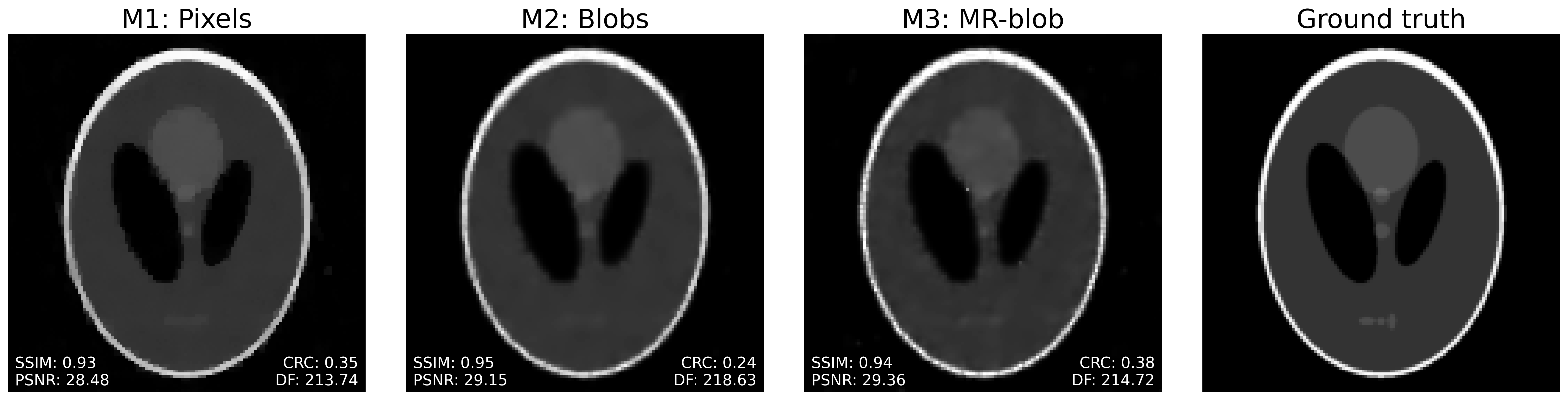
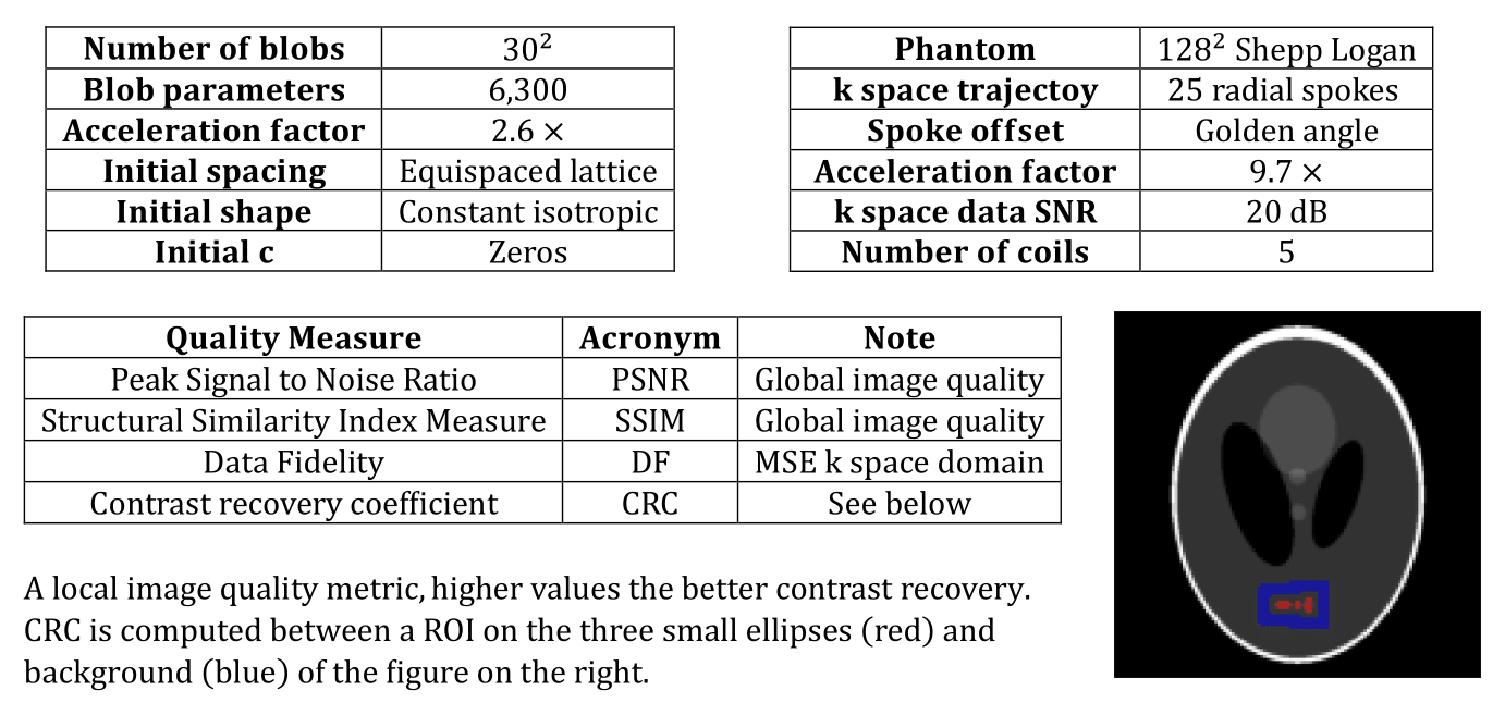
Results: Noisy, undersampled parallel MRI simulations of Shepp-Logan phantom are reconstructed with a pixelised image, a coordinate-transformed blob-based image, and MR-blob; all with total variation regularisation. Quality measures are shown to be consistent across methods and regularisation strengths.
Impact: Parameter-efficient image representations have the potential to reduce computational burden. This work defines parallel MRI forward model for coordinate-transformed blobs. This includes auto-calibrating coil sensitivities that re-scale and translate to fit the parallel MRI measurements.
Introduction
Images are functions defined on two continuous spatial coordinates $$$r_x$$$ and $$$r_y$$$, and are discretised to allow for digital processing. The most prevalent discretisation is via equally-spaced piece-wise-constant basis functions, aka pixels. Other local basis functions have been developed1 and applied to image reconstruction.2,3 This work investigates the use of Gaussian functions, herein referred to as blobs. These blobs are locally defined, and to globally represent an image a set of blobs is typically fixed as an equally-spaced lattice of specific scale. Recently, Gaussian splats were proposed4 that parameterise and optimise the covariance of the blobs. This was shown to be effective and efficient for radiance field rendering. We re-parameterise Gaussian splats as coordinate-transformed blobs. Using such coordinate-transformed blobs, we develop a forward model to reconstruct parallel MRI measurements and auto-calibrate the coil sensitivities; this is termed as MR-blob.Coordinate-transformed blobs
We consider coordinate transformed blobs of the form:\begin{align}b(\mathbf{r})&=b(\mathbf{r};c,\mathbf{T},\mathbf{t})=c\exp{\left(-\frac{1}{2}\hat{\mathbf{r}}(\mathbf{r})^\top\hat{\mathbf{r}}(\mathbf{r})\right)},~\text{for}~\hat{\mathbf{r}}(\mathbf{r})=\mathbf{T}\mathbf{r}+\mathbf{t}=\begin{bmatrix}s^{x,x}&s^{x,y}\\s^{y,x}&s^{y,y}\\\end{bmatrix}\begin{bmatrix}r_x\\r_y\end{bmatrix}+\begin{bmatrix}t_x\\t_y\end{bmatrix},\end{align}where $$$\mathbf{r}=[r_x,~r_y]^\top$$$ is the coordinate system, and $$$c$$$ the contrast. Herein $$$\mathbf{T}$$$ is a general linear transform of the coordinate system, and $$$\mathbf{t}$$$ is translation.A coordinate transformed blob can be rewritten as:\begin{equation}b(\mathbf{r})=c\mathcal{N}(\mathbf{r};-\mathbf{T}^{-1}\mathbf{t},(\mathbf{T}^\top \mathbf{T})^{-1}),\end{equation}where $$$\mathcal{N}(\mathbf{r};\mu,\Sigma)=\exp\left(-\frac{1}{2}(\mathbf{x}-\mu)^{\top}\Sigma^{-1}(\mathbf{x}-\mu)\right)$$$ is the un-normalised Gaussian function with mean $$$\mu$$$ and covariance $$$\Sigma$$$. To represent more complex functions, e.g., images, an ensemble of blobs is used:\begin{equation}B(\mathbf{r})=B(\mathbf{r};C,\Phi):=\sum_{i=1}^{N_b}b(\mathbf{r};c_i,\mathbf{T}_i,\mathbf{t}_i).\end{equation} We define $$$C=\{c_i\}_{i=1}^{N_b}$$$ as contrast and $$$\Phi=\{(\mathbf{T}_i,\mathbf{t}_i)\}_{i=1}^{N_b}$$$ as the basis of the coordinate-transformed blobs.Single coil modelling
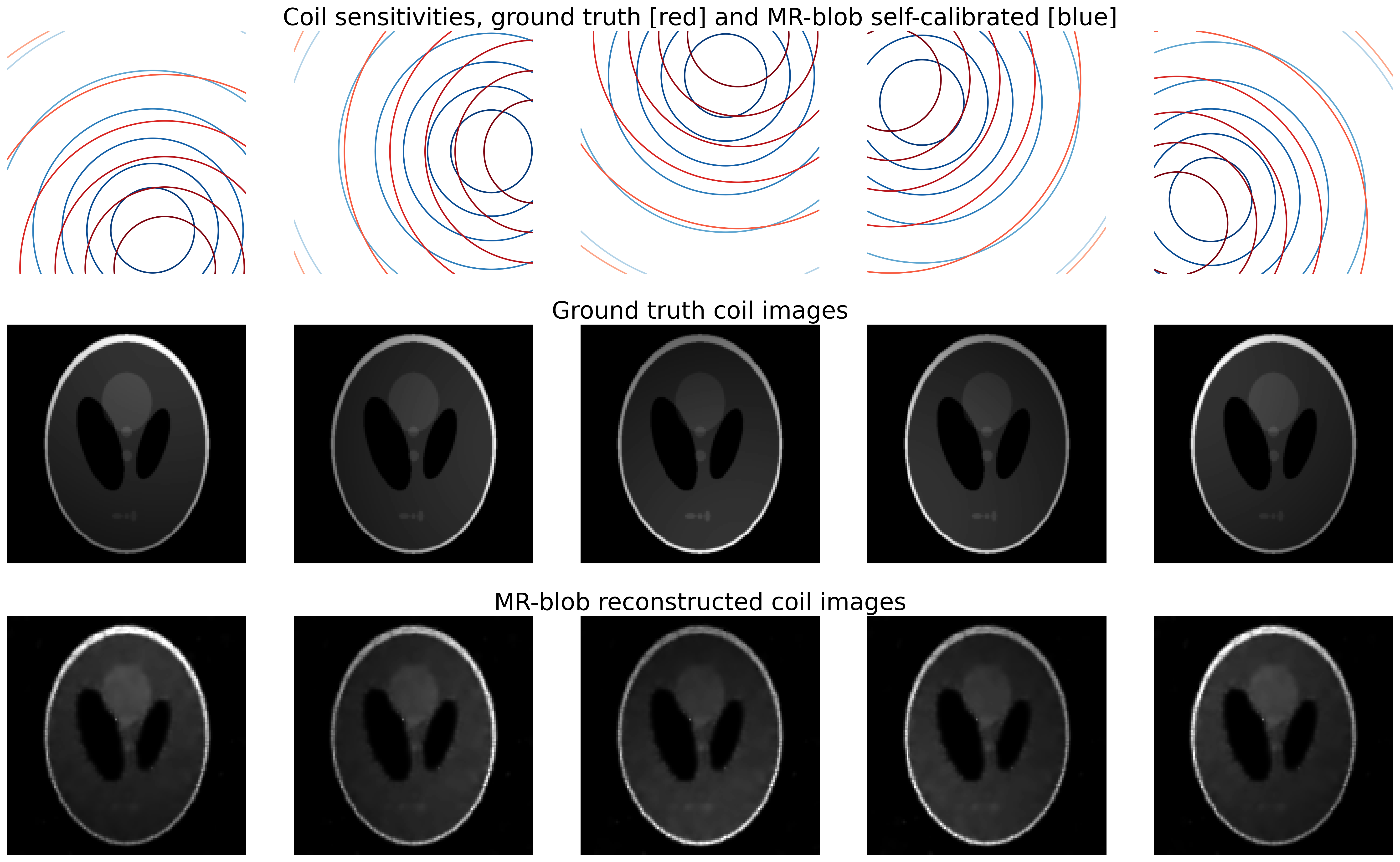
Coil sensitivities are modelled as un-normalised isotropic Gaussians:\begin{equation*}b_\kappa(\mathbf{r})=b_{\kappa}(\mathbf{r};s_{\kappa},\mu_{\kappa}):=\mathcal{N}(\mathbf{r};\mu_\kappa,s_\kappa^2\mathbf{I})\end{equation*}with scale $$$s_\kappa$$$ and centre $$$\mu_\kappa$$$. The coil sensitivity acts such that signal closer to the centre is stronger and decays in space exponentially. A coil image, the coil sensitivities on the image, is modelled as:5$$b_{\kappa}(\mathbf{r}; s_{\kappa},\mu_{\kappa})\cdot B(\mathbf{r};C,\Phi)=\sum_{i=1}^{N_b}k_{\kappa,i}\mathcal{N}\left(\mathbf{r}, \mu_{\kappa,i},\Sigma_{\kappa,i}\right),$$where\begin{equation}\begin{split}\Sigma_{\kappa,i}&=(\mathbf{T}_i^\top\mathbf{T}_i+s_\kappa^2\mathbf{I}),\quad\mu_{\kappa,i}=\Sigma_{\kappa,i}^{-1}(-\mathbf{T}_i^\top\mathbf{t}_i+s_\kappa^2\mu_\kappa),\quad\\k_{\kappa,i}&=c_i\sqrt{\det(\Sigma_{\kappa,i}^{-1})} \exp\left(-\frac{1}{2}(-\mathbf{T}^{-1}_i\mathbf{t}_i-\mu_\kappa)^\top\Sigma_{\kappa,i}^{-1}(-\mathbf{T}^{-1}_i\mathbf{t}_i-\mu_\kappa)\right)\end{split}\end{equation}MRI measurements acquired by a coil are in the frequency (k-space) domain. These can be modelled in k-space coordinates $$$\mathbf{k} = [k_x,~ k_y]^\top$$$ by Fourier transforming $$$b_\kappa(\mathbf{r}) \cdot B(\mathbf{r})$$$:\begin{align}\mathcal{F}\{b_{\kappa}(\mathbf{r};s_{\kappa},\mu_{\kappa})\cdot B(\mathbf{r};C,\Phi)\}(\mathbf{k})&=\mathcal{F}\{k_{\kappa,i}\mathcal{N}(\mathbf{r};\mu_{\kappa,i},\Sigma_{\kappa,i})\}(\mathbf{k})\\&=\sum_{i=1}^{N_b}\frac{2\pi k_{\kappa,i}}{\sqrt{\det(\Sigma_{\kappa,i})}}\exp\left(-i\mathbf{k}^\top\mu_{\kappa,i}-\frac{1}{2}\mathbf{k}^\top\Sigma_{\kappa,i}\mathbf{k}\right).\end{align}MR-blob: formulation and inverse problem
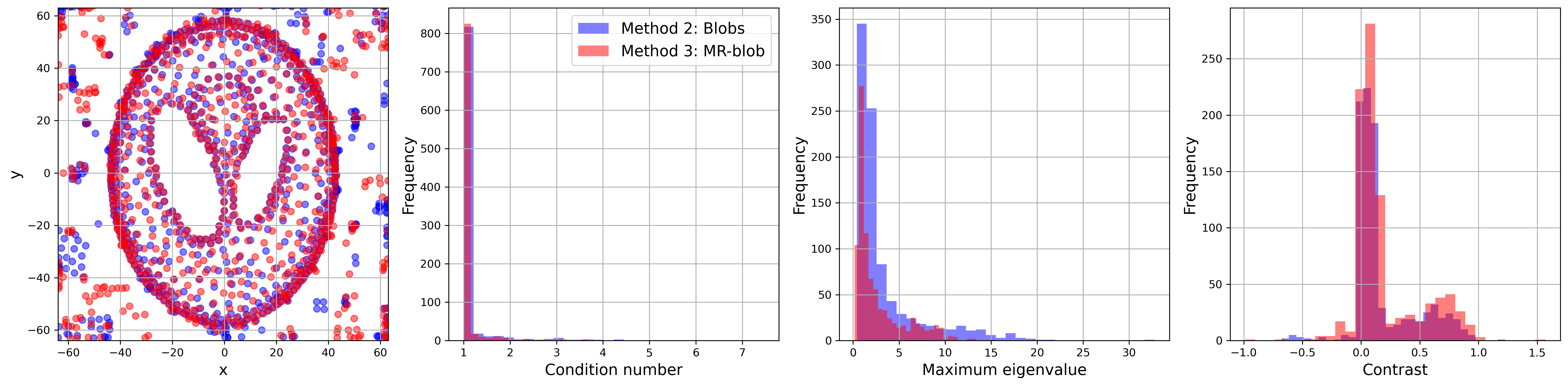
We define the MR-blob as:\begin{equation}\text{MR-blob}(\mathbf{k};S,M,C,\Phi):=\begin{pmatrix}\mathcal{F}(b_{1}(\mathbf{r};s_{{1}},\mu_{1})\cdot B(\mathbf{r};C,\Phi))(\mathbf{k})\\\vdots\\\mathcal{F}(b_{{N_{\kappa}}}(\mathbf{r};s_{{N_{\kappa}}},\mu_{{N_{\kappa}}})\cdot B(\mathbf{r};C,\Phi))(\mathbf{k})\end{pmatrix}.\end{equation}The parameters of the coils are scales $$$S:=\{s_\kappa\}_{\kappa=1}^{N_{\kappa}}$$$ and centres $$$M:=\{\mu_\kappa\}_{\kappa=1}^{N_{\kappa}}$$$. The same contrast $$$C$$$ and basis $$$\Phi$$$ are used across all coils. The inverse problem is given by:$$\text{MR-blob}(\mathbf{k};S,M,C,\Phi) = G(\mathbf{k}),$$where parallel MRI measurements are $$$G: \Omega_k \mapsto \mathbb{C}^{N_\kappa}$$$ with $$$N_\kappa\in\mathbb{N}$$$ coils. The domain $$$\Omega_k = \{ \mathbf{k}_n \}_{n=1}^{N_k}$$$ is a set of coordinates with $$$N_k\in\mathbb{N}$$$ measurements.In the variational framework of inverse problems,6 we recover the parameters of the reconstruction through optimising:\begin{equation}S^*,M^*,C^*,\Phi^*\in\min_{S,M,C,\Phi}\left\{\frac{1}{N_k}\sum_{n=1}^{N_k}||\text{MR-blob}(\mathbf{k}_n;S,M,C,\Phi)-G(\mathbf{k}_n)||^2+\lambda R(B(\mathbf{r};C,\Phi))\right\},\end{equation}where the first term promotes data-consistency, and the second is a regulariser with strength $$$\lambda$$$. We directly optimise over blob parameters (contrast $$$C$$$ and basis $$$\Phi$$$), as well as over the coil sensitivities, specified by $$$S$$$ and $$$M$$$. Thus, we jointly reconstruct the image and calibrate the coil sensitivities. The reconstruction $$$f:\Omega_r\mapsto\mathbb{C}~\text{with}~\Omega_r=\{ \mathbf{r}_m\}_{m=1}^{N_r}$$$ is given by\begin{equation}f(\mathbf{r})=B(\mathbf{r};C^*,\Phi^*).\end{equation}We study two regularisers:\begin{align}R_{\text{cond}}(\Phi):=&\frac{1}{N_{b}}\sum_{i=1}^{N_{b}}\text{cond}(\mathbf{T}_i^{\top}\mathbf{T}_i),\\R_{\text{TV}}(\Omega_r;C,\Phi):=&\frac{1}{N_{r}}\sum_{m=1}^{N_r} R_{\text{TV}}(\mathbf{r}_m;C,\Phi), \text{ with }R_{\text{TV}}(\mathbf{r};C,\Phi):=\|\nabla_{\mathbf{r}}B(\mathbf{r};C,\Phi)\|_1, \end{align}promoting blob skewness and TV sparsity, respectively. We optimise the variational objective by taking the gradients using automatic (reverse-mode) differentiation with the first-order ADAM optimiser.7Methods
Three methods were compared to illustrate the features of reconstruction with pixels (M1), blobs (M2) and MR-blobs (M3). We denote the pixelised image as $$$\mathbf{f}\in\mathbb{C}^{N_r}$$$, and Non-Uniform-Fast-Fourier-Transform (NUFFT) with coil sensitivities forward model as $$$\mathbf{A}:\mathbb{C}^{N_r}\mapsto\mathbb{C}^{N_k\times N_\kappa}$$$. The corresponding objective functions are given by\begin{align}\text{M1 (Pixels):}&~\min_{\mathbf{f}}\left\{\frac{1}{N_k}||\mathbf{A} \mathbf{f}-G(\Omega_k)||_F^2+\frac{\lambda}{N_r}||\nabla\mathbf{f}||_1\right\}\\\text{M2 (Blobs):}&~\min_{C,\Phi}\Bigg\{\frac{1}{N_k}||\mathbf{A}B(\Omega_r;C,\Phi)-G(\Omega_k)||_F^2+10\cdot R_{\text{cond}}(\Phi)+\lambda R_{\text{TV}}(\Omega_r;C,\Phi)\Bigg\}\\\text{M3}~\text{(MR-blob):}&~\min_{S,M,C,\Phi}\Bigg\{\frac{1}{N_k}\sum_{n=1}^{N_k}||\text{MR-blob}(\mathbf{k}_n;S,M,C,\Phi)-G(\mathbf{k}_n)||^2\nonumber\\&\qquad\qquad\qquad\qquad\qquad+10\cdot R_{\text{cond}}(\Phi)+\lambda R_{\text{TV}}(\Omega_r;C,\Phi)\Bigg\},\end{align}where $$$G(\Omega_k) := [G(\mathbf{k}_1),\ldots,G(\mathbf{k}_{N_k})]$$$ and $$$B(\Omega_r;C,\Phi):=[B(\mathbf{r}_1;C,\Phi),\ldots,B(\mathbf{r}_{N_r};C,\Phi)]^{\top}$$$. TV regularisation with the same $$$\lambda$$$s were tested for all three methods. For M2 and M3 we include a constant skew-penalisation and evaluate TV at points corresponding to pixel centres.Discussion and Conclusion
The same forward model used for simulation is used for reconstruction for M1 and M2. With coil sensitivities of MR-blob initially centred in the image, auto-calibration allows the coils to translate and re-scale to fit to measurements. This resulted in coil sensitivities and coil image shown in Fig. 5. Further, the piece-wise-constant structure of the Shepp-Logan phantom is not well approximated by smooth basis functions such as blobs. Notwithstanding, it is observed that blob-based images give competitive performance with $$$2.6\times$$$ less parameters than pixels. Additionally, the smoothness of blobs provides implicit regularisation at lower regularisation values. The M2 and M3 reconstructions exhibit bases $$$\Phi$$$ with prominent structure, see Fig. 4. It is noted that M3 gave fewer zero contrasts, less skewed blobs and a larger range of scales compared to M2.The data-consistency terms of M2 and M3 are smooth given positive-definite covariances, but highly non-convex. The optimisation could benefit from more specialised algorithm. This will be investigated further where acceleration would benefit scaling to 3D in-vivo measurements. We have shown coordinate-transformed blobs are able to approximate parallel MRI reconstructions efficiently and accurately. Given the simplicity of the formulation it is amenable to rigorous analysis, and we leave that for future work.
Acknowledgements
I.R.D. Singh was supported by the EPSRC-funded UCL Centre for Doctoral Training in Intelligent, Integrated Imaging in Healthcare (i4health) (EP/S021930/1) and the Department of Health’s NIHR-funded Biomedical Research Centre at University College London Hospitals. Ž. Kereta was supported by the UK EPSRC grant EP/X010740/1. A. Denker was supported by the Deutsche Forschungsgemeinschaft (DFG, German Research Foundation) - Project number 281474342/GRK2224/2. B. Jin and S. Arridge were supported by the UK EPSRC EP/V026259/1. The authors would like to thank Mark Griswold and Peter J. Lally for their fruitful discussion.References
1. Hanson, Kenneth M., and George W. Wecksung. "Local basis-function approach to computed tomography." Applied Optics 24.23 (1985): 4028-4039.
2. Lewitt, Robert M. "Alternatives to voxels for image representation in iterative reconstruction algorithms." Physics in Medicine & Biology 37.3 (1992): 705.
3. Schweiger, Martin, and Simon R. Arridge. "Image reconstruction in optical tomography using local basis functions." Journal of Electronic Imaging 12.4 (2003): 583-593.
4. Kerbl, Bernhard, et al. "3D gaussian splatting for real-time radiance field rendering." ACM Transactions on Graphics (ToG) 42.4 (2023): 1-14.
5. Petersen, Kaare Brandt, and Michael Syskind Pedersen. "The matrix cookbook." Technical University of Denmark 7.15 (2008): 510.
6. Scherzer, Otmar, et al. "Variational methods in imaging." Vol. 167. Springer Science+ Business Media LLC, 2009.
7. Kingma, Diederik P., and Jimmy Ba. "Adam: A method for stochastic optimization." arXiv preprint arXiv:1412.6980 (2014).
Figures
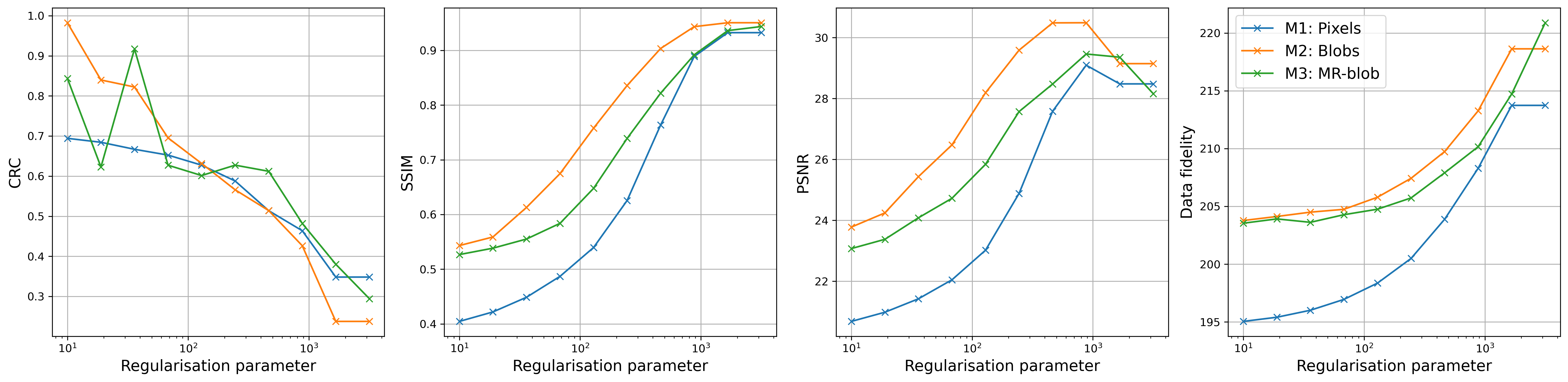
CRC, SSIM, PSNR, DF for all three methods swept over the same range of regularisation parameters ($$$\log_{10}(\lambda)\in$$${1.00,1.28,1.56,1.83,2.11,2.39,2.67,2.94,3.22,3.50})