1859
Artifact Simulation Toolbox for GABA-Edited Magnetic Resonance Spectroscopy1Department of Biomedical Engineering, University of Calgary, Calgary, AB, Canada, 2Department of Radiology, University of Calgary, Calgary, AB, Canada, 3Hotchkiss Brain Institute, University of Calgary, Calgary, AB, Canada, 4Alberta Children's Hospital Research Institute, University of Calgary, Calgary, AB, Canada, 5Department of Electrical & Software Engineering, University of Calgary, Calgary, AB, Canada
Synopsis
Keywords: Spectroscopy, Spectroscopy, Software Tools, Simulations, Artifacts, Brain
Motivation: GABA-edited Magnetic Resonance Spectroscopy (MRS) is a valuable tool used to measure GABA. However, it suffers from low signal to noise ratio. Machine learning has been recently proposed to overcome these challenges but accessing the large amount of in vivo data necessary for training can be difficult.
Goal(s): To create a GABA-edited MRS artifact toolbox.
Approach: We developed an open-access python toolbox to simulate four common artifacts (ghosting, eddy current effects, lipid contamination and phase/frequency shifts) in GABA-edited MRS.
Results: The toolbox will support machine learning algorithm development by complementing existing simulation software and allow for flexible user inputs for data personalization.
Impact: Our open-access python toolbox can be used to simulate spurious echoes, eddy currents, lipid contamination and motion artifacts to provide realistic and representative GABA-edited MRS data. This can be used for methods development such as training machine learning algorithms.
INTRODUCTION
Edited-MRS data suffers from poor data quality1. This is further challenged in clinical populations with low scanner tolerance, often resulting in excessive motion leading some studies to reject up to 10% of their datasets2,3. As methods are developed to address data quality, including machine learning based approaches4-10, so does the need for adequate simulations. To address this need, we propose an open-access python toolbox to simulate commonly occurring artifacts in GABA-edited MRS data with potential use for method development, machine learning models or for software development.METHODS: FRAMEWORK FOR SIMULATION SOFTWARE
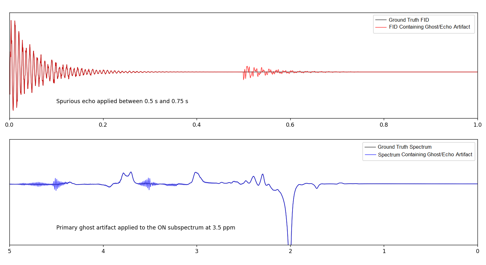
An arbitrary number of Edit-ON/Edit-OFF transients can be simulated from ground truth spectra11 to represent a single scan. Gaussian white noise and random frequency and phase shifts are then added to represent the quality of a typical scan (SNR of ~25)12. A random subset of the following artifacts is then generated individually or in combination and inserted into the scan.Ghosting or Spurious Echoes Artifacts13,14 are simulated in the time domain and are modelled using the following equation:
$$FID(t)=\begin{cases}FID_0&t<t_s\ or\ t>t_f\\FID_0\times A\times e^{\frac{-t}{T_{all}}}\times e^{-j\times\left(t\times lf\times\left(1-Cs\right)+\theta\right)}&t_s\leq t\leq t_f\end{cases}\tag{1}$$
where t is the time of the FID, ts and tf define the start and end time of the artifact, FID_0 contains the current values of the time domain signal as function of time, A is the amplitude of the artifact, T_all is the length in seconds of the FID, lf is the Larmor frequency of hydrogen in Hz, Cs is the position of the artifact in ppm in the frequency domain, and θ is the phase of the artifact in radians.
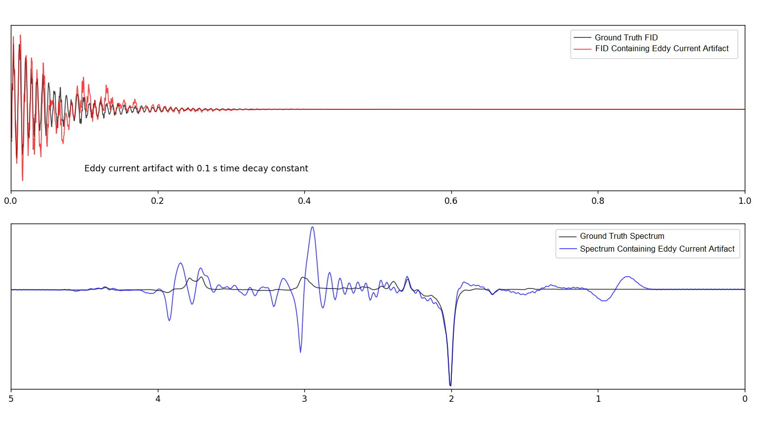
Eddy Current (EC) Artifacts can occur despite hardware solutions, particularly with highly selective editing pulses14,15. EC artifacts are simulated in the time domain and are modelled by:
$$FID(t)=FID_0\times e^{-j\times 2\pi t\times A\times e^{\frac{t}{t_c}}}\tag{2}$$
where t is the time of the FID, FID_0 contains the current values of the time domain signal, A is the amplitude of the artifact and tc is the time constant in seconds of the decaying artifact.
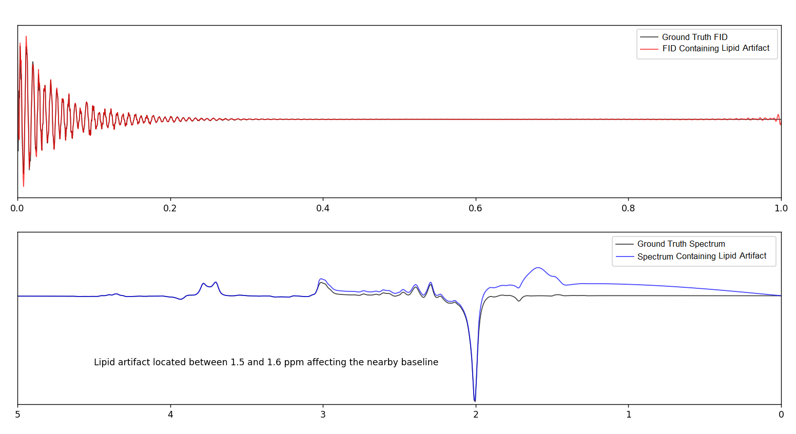
Lipid Contamination Artifacts overlap metabolites of interest, making their removal difficult14. Lipid contamination is simulated in the frequency domain and includes baseline change (Eq.3) and peak simulation (Eq.4).
$$Spec(f)=\begin{cases}Spec_0&f<f_s\ or\ f>f_f\\Spec_0+|A\times sin(B\times f)|&f_s\leq f\leq f_f\end{cases}\tag{3}$$
$$Spec(f)=\begin{cases}Spec_0&f<f_s\ or\ f>f_f\\Spec_0+(A_1\times e^{-(f-f_1)^2})+(A_2\times e^{-(f-f_2)^2})&f_s\leq f\leq f_f\end{cases}\tag{4}$$
where f contains the frequency axis values, fs and ff denote the start and end frequencies of the artifact, Spec_0 contains the current spectral domain values of the signal as function of frequency, A is the amplitude of the baseline, B represents the period of the sine wave, A1 and A2 are the amplitudes of the overlapping Gaussians simulating the lipid peak contamination, and f1 & f2 are the locations of these peaks.
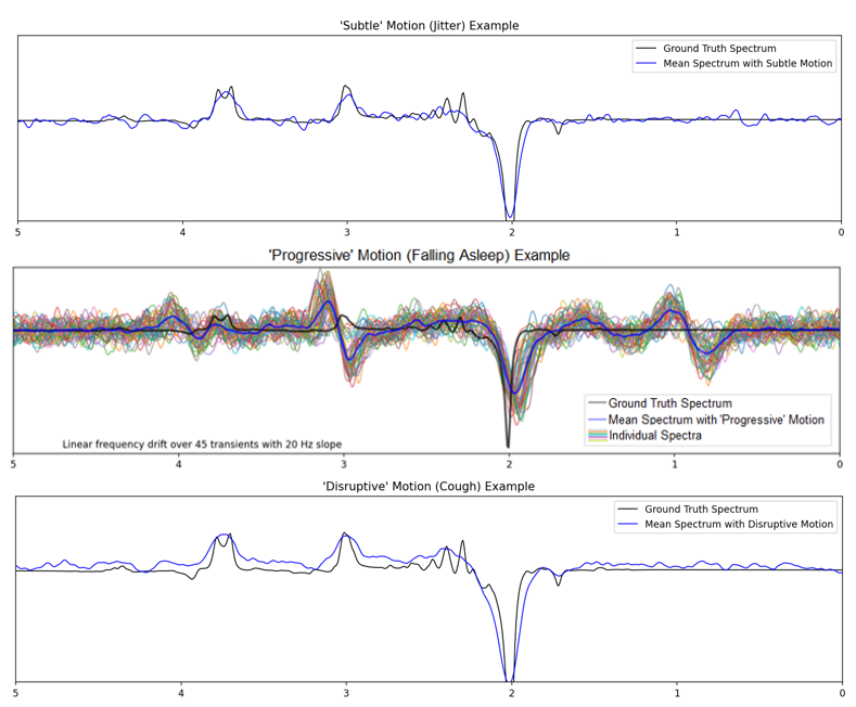
Motion Contamination Artifacts occur in a range of different ways14. We have defined three main categories of motion artifact:
- ‘Subtle’: small discrete motions (e.g., jittering/fidgeting) throughout the scan, resulting in random frequency and phase shifts.
- ‘Progressive’: slow systematic motion throughout the scan (e.g., head drifting as a subject falls asleep or small thermal variations), primarily resulting in a long, linear frequency drift.
- ‘Disruptive’: large, single, discrete motion (e.g., cough) affecting only a few subspectra primarily by line broadening and baseline change.
Baseline change (Eq. 3), random frequency shifts (Eq.5), random phase shifts (Eq. 6), linear frequency drifts (Eq. 7), line broadening (Eq. 8) are shown below:
$$FID(t)=FID_0\times e^{j\times2\pi t\times noise_{frequency}}\tag{5}$$
$$FID(t)=FID_0\times e^{j\times\frac{\pi}{180}\times noise_{phase}}\tag{6}$$
$$FID(t)=FID_0\times e^{j\times2\pi t\times noise_{linear}}\tag{7}$$
$$FID(t)=FID_0\times A\times e^{-t\times lvs}\tag{8}$$
where t is the time of the FID, FID_0 contains the current values of the time domain signal as function of time, noisefrequency and noisephase are a set of random normally distributed values with mean 0 and standard deviation set by the user, noiselinear is a set of normally distributed values with mean 0, standard deviation and slope set by the user, and lvs is the lineshape variance, and A is amplitude of the artifact.
The above-mentioned artifacts can be simulated alone or in combination and can be simulated in any order.
RESULTS
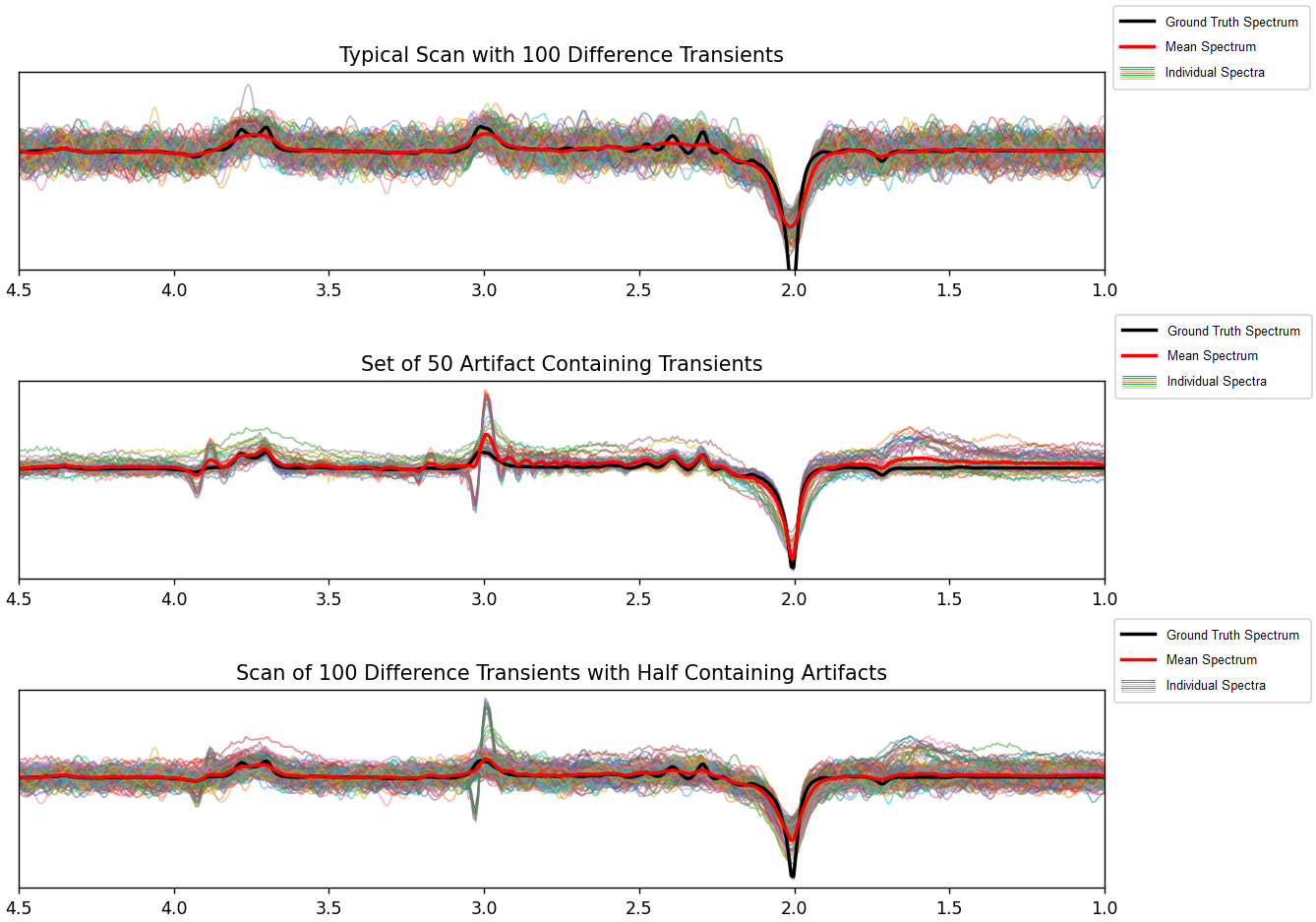
Example spectra of the simulated artifacts individually and in combination in both the time and frequency domains are shown in Figures 1-5.CONCLUSION
The toolbox maximizes flexibility, allowing for a change in the individual artifact parameters, the number of corrupted transients, the location of corrupted transients within a scan, and the option to simultaneously simulate multiple artifacts.This toolbox complements existing simulation software by enabling users to simulate commonly occurring artifacts seen in GABA-edited MRS data, which can be used to support the development of machine learning algorithms.
The toolbox is available at https://github.com/HBugler/GABA-Edited-Artifact-Simulation-Toolbox.git.
Acknowledgements
HB was supported by NSERC Brain CREATE Award and Alberta Graduate Excellence Scholarship. RS was supported by NSERC Discovery Grant (#RGPIN-2021-02867) and AH was supported by NSERC Discovery Grant (# RGPIN-2017-03875).References
- Mullins PG, McGonigle DJ, O’Gorman RL, et al. Current practice in the use of MEGA-PRESS spectroscopy for the detection of GABA. NeuroImage. 2014; 86:43-52.
- Bell TK, Stokoe M, Akashroop K, et al. GABA and glutamate in pediatric migraine. Pain. 2021; 162(1):300-308.
- La PL, Joyce JM, Bell TK, et al. Brain metabolites measured with magnetic resonance spectroscopy in pediatric concussion and orthopedic injury: An Advancing Concussion Assessment in Pediatrics (A-CAP) study. Hum. Brain Mapp. 2023; 44(6):2493-2508.
- Bugler H, Berto RP, Souza R, and Harris AD. Frequency and Phase Correction of GABA-Edited Magnetic Resonance Spectroscopy using Complex-Valued Convolutional Neural Networks. bioRxiv, 2023.
- Tapper S, Mikkelsen M, Dewey BE, et al. Frequency and phase correction of J-difference edited MR spectra using deep learning. Magn Reson Med. 2021;85(4):1755-1765.
- Ma DJ, Le HAM, Ye Y, et al. MR spectroscopy frequency and phase correction using convolutional neural networks. Magn Reson Med. 2022;87(4):1700-1710.
- Rakic M, Turco F, Weng G, Maes F, Sima DM, and Slotboom J. Deep learning pipeline for quality filtering of MRSI spectra. NMR Biomed. 2023: e.5012.
- Jang J, Hun Lee H, Park JA, and Kim H. Unsupervised anomaly detection using generative adversarial networks in 1H-MRS of the brain. J. Magn. Reson. 2021;325: 106936.
- Shamaei A, Starcukova J, and Starcuk Jr. Z. Physics-informed deep learning approach to quantification of human brain metabolites from magnetic resonance spectroscopy data. Comput Biol Med. 2023; 158: 106837.
- Zhang Y, and Shen J. Quantification of spatially localized MRS by novel deep learning approach without spectral fitting. Magn Reson Med. 2023; 90(4): 1282-1296.
- Simpson R, Devenyi GA, Jezzard P, Hennessy TJ, and Near J. Advanced processing and simulation of MRS data using the FID applicance (FID-A) - An open source, MATALAB-based toolkit. Magn Reson Med. 2017;77(1):23-33.
- Mikkelsen M, Barker PB, Bhattacharyya PK, et al. Big GABA: Edited MR Spectroscopy at 24 Research Sites. NeuroImage. 2017;159(32-45):32-45.
- Berrington A, Povazan M, and Barker PB. Estimation and removal of spurious echo artifacts in single-voxel MRS using sensitivity encoding. Magn Reson Med. 2021;86(5): 2339-2352.
- Kreis R. Issues of spectral quality in clinical 1H-magnetic resonance spectroscopy and a gallery of artifacts. NMR Biomed. 2004; 17(6):361-81.
- Oeltzschner G, Snoussi K, Puts NAJ, et al. Effects of eddy currents on selective spectral editing experiments at 3T. J Magn Reason Imaging. 2018;47(3):673-681.
Figures