1768
PEARL: Cascaded Self-supervised Cross-fusion Learning For Parallel MRI Acceleration
Qingyong Zhu1, Bei Liu2, Zhuo-Xu Cui1, Chentao Cao3, Xiaomeng Yan2, Yuanyuan Liu3, Jing Cheng3, Yihang Zhou1, Yanjie Zhu3, Haifeng Wang3, Hongwu Zeng4, and Dong Liang1
1Research Center for Medical AI, SIAT, Chinese Academy of Sciences, Shenzhen, China, 2School of Mathematics, Northwest University, Xi'an, China, 3Paul C. Lauterbur Research Center for Biomedical Imaging, SIAT, Chinese Academy of Sciences, Shenzhen, China, 4Shenzhen Children’s Hospital, Shenzhen, China
1Research Center for Medical AI, SIAT, Chinese Academy of Sciences, Shenzhen, China, 2School of Mathematics, Northwest University, Xi'an, China, 3Paul C. Lauterbur Research Center for Biomedical Imaging, SIAT, Chinese Academy of Sciences, Shenzhen, China, 4Shenzhen Children’s Hospital, Shenzhen, China
Synopsis
Keywords: AI/ML Image Reconstruction, Image Reconstruction, Self-supervised AI
Motivation: Supervised deep learning (SDL) has limitations due to data dependency, and self-supervised frameworks like DIP struggle with noise and artifacts.
Goal(s): Introducing PEARL, a novel self-supervised accelerated parallel MRI approach.
Approach: PEARL leverages joint deep decoders coupling with cross-fusion schemes based on multi-parameter priors to achieve enhanced reconstruction.
Results: PEARL outperforms the existing methods, demonstrating notable improvement under highly accelerated acquisition.
Impact: This study emphasizes the significance and potential of self-supervised learning in addressing critical MRI challenges.
Introduction
Comprising encoder and decoder, the DIP $$$^{1}$$$ serves as a deep network prior-based image generator. For accelerated MRI (AMRI) problem, the DIP aims to minimize the function,$$\begin{equation} \theta^{*}\in\mathop{\arg\min}_{\theta\in\mathbb{R}^p}\frac{1}{2}\sum_{s=1}^{E}\parallel\!A_{s}\left(\phi_{\theta}(\eta)\right)_{s}-y_{s}\!\parallel_{2}^{2}\!\end{equation}$$where $$$\eta\in\mathbb{R}^p$$$ is a fixed parameter vector. $$$\phi_{\theta}:\mathbb{R}^p \rightarrow \mathbb{R}^{c\times w\times h}$$$ serves as a mapping. $$$\theta$$$ denotes the learned parameters. $$$c$$$ is the number of channels, and $$$w,h$$$ are the width and height, respectively. $$$s$$$ and $$$E$$$ denote the coil index and the total number of coils, respectively.
Method
The proposed PEARL approach is built upon a multi-stream joint deep decoder that integrates additive and multiplicative cross-fusion learning for multi-parameter priors $$$^{2,3,4,5}$$$. Each stream contains cascaded cross-fusion SBNs. One SBN performs combined upsampling $$${U}\left(\cdot,\cdot\right)$$$ , 2D convolution $$$C(\cdot)$$$, joint attention $$$J\left(\cdot,\cdot\right)$$$, ReLU activation $$$\sigma(\cdot)$$$ and BN $$$B\left(\cdot\right)$$$. The detailed two-stream network architecture is illustrated in Figure 1. Specifically, the inputs are the two fixed random vectors $$$\eta_{i:i=1,2}\in\mathbb{R}^{1 \times {2} \times {w_{in}}\times {h_{in}}}$$$ and the outputs are the generated images $$$\rho_{{i}:i=1,2}\in\mathbb{R}^{1 \times {{2E} \times {w_{out}} \times {h_{out}}}}$$$. The final estimated images $$$\hat{x}_{i:i=1,2}$$$ are derived through data consistency and channel synthesis. Then, for the cross-fusion $$${\rm{SBN}}_{k}$$$, the two-stream outputs $$$F_{{1}}^{k}\in{\mathbb{R}^{1\times {c^k}\times {w^k}\times {h^k}}}$$$ and $$$F_{{2}}^{k}\in {\mathbb{R}^{1 \times {c^k} \times {w^k} \times {h^k}}} ({w^k} = {w_{in}} \cdot {2^{k}}, {h^k} = {h_{in}} \cdot {2^{k}}, k\geq 1)$$$ are described as follows,$$\begin{equation} { F_{{1}}^{k}= B_{1}\left(\sigma_{1}\left({J_{1}^{k}}\left(C^{k}_{1}\left(U_{1}^{k}\left(F_{1}^{k-1}\right) \right),C^{k}_{2}\left(U_{2}^{k}\left(F_{{2}}^{k-1}\right)\right)\right)\right)\right)}\end{equation}$$,$$\begin{equation} { F_{{2}}^{k}= B_{2}\left(\sigma_{2}\left({J_{2}^{k}}\left(C^{k}_{2}\left(U_{2}^{k}\left(F_{2}^{k-1}\right) \right),C^{k}_{1}\left(U_{1}^{k}\left(F_{{1}}^{k-1}\right)\right)\right)\right)\right)}\end{equation}$$where $$$F_{i:i=1,2}^{0}=\eta_{i:i=1,2}$$$. Firstly, we developed a combined upsampling strategy. Specifically, the combined upsampling for the $$$p$$$-th pixel of the $$${t}$$$-th feature maps in the $$${\rm{SBN}}_{k}$$$ layers is defined as follows,$$\begin{equation} \small{ \begin{aligned} \left(U_{1}^{k}\left(F_{{1}}^{k}\right)\right)_{t,p}= &\sum_{q\in R(p)}\alpha_{1}^{k}(p,q)\circ\left(\uparrow_{bic}\left(F_{{1}}^{k}\right)\right)_{t,q}\\ +&\sum_{q\in R(p)}\beta_{1}^{k}(p,q)\circ\left(\uparrow_{bic}\left(F_{{2}}^{k}\right)\right) _{t,q} \end{aligned}}\end{equation}$$$$\begin{equation} \small{ \begin{aligned} \left(U_{2}^{k}\left(F_{{2}}^{k}\right)\right)_{t,p}= &\sum_{q\in R(p)}\alpha_{2}^{k}(p,q)\circ\left(\uparrow_{bic}\left(F_{{2}}^{k}\right)\right)_{t,q}\\ +&\sum_{q\in R(p)}\beta_{2}^{k}(p,q)\circ\left(\uparrow_{bic}\left(F_{{1}}^{k}\right)\right)_{t,q} \end{aligned}}\end{equation}$$where $$$\uparrow_{bic}\!(\cdot)$$$ is the $$$\textit{bicubic}$$$ upsampling. $$$R(p)$$$ denotes the pixel set in the patch centered at $$$p$$$. $$$\alpha_{1}^{k}(p,q)$$$, $$$\alpha_{2}^{k}(p,q)$$$, $$$\beta_{1}^{k}(p,q)$$$ and $$$\beta_{2}^{k}(p,q)$$$ represent the learnable parameters. Secondly, the joint attention is further designed. Specifically, the joint attention in the cross-fusion $$${\rm{SBN}}_{k}$$$ is defined as follows, $$\begin{equation}\begin{aligned}{} J_{{1}}^{k}\left(\widetilde{F_{{1}}^{k}}\right) = \widetilde{F_{{1}}^{k}} + \left({w_{{1},CA}}\circ w_{{2},CA}\right) \circ \widetilde{F_{{1}}^{k}} + \left({w_{{1},SA}}\circ w_{{2},SA}\right) \circ \widetilde{F_{{1}}^{k}}\\ J_{{2}}^{k}\left(\widetilde{F_{{2}}^{k}}\right) = \widetilde{F_{{2}}^{k}} + \left({w_{{1},CA}}\circ w_{{2},CA}\right) \circ \widetilde{F_{{2}}^{k}}+\left({w_{{1},SA}}\circ w_{{2},SA}\right) \circ \widetilde{F_{{2}}^{k}} \end{aligned}\end{equation}$$where $$$\widetilde{F_{{1}}^{k}}=C^{k}_{1}\left(U_{1}^{k}\left(F_{{1}}^{k}\right)\right)$$$ and $$$\widetilde{F_{{2}}^{k}}=C^{k}_{2}\left(U_{2}^{k}\left(F_{{2}}^{k}\right)\right)$$$. Notably, the corresponding channel and spatial weights $$$w_{1,CA}$$$, $$$w_{1,SA}$$$, $$$w_{2,CA}$$$ and $$$w_{2,SA}$$$ that are multiplied together highlight or suppress feature maps. Besides, to prevent vanishing gradients, a long-range unified skip connection $$$^{6}$$$ is established to capture and propagate information across distant layers. In addition to utilizing the loss functions based on data fitting of two target images, we newly designed a regularization loss based on the dual-normalized edge-orientation similarity, that is, $$\begin{equation}\begin{aligned} L(\theta_{1},\theta_{2})= \sum_{s=1}^{E}\parallel y_{1,s}-A_{1,s}\left(\phi_{\theta_{1}}\left(\eta_{1}\right)\right)_{s}\parallel_{\rm{2}}^{2} +\lambda\sum_{s=1}^{E}\parallel y_{2,s}-A_{2,s}\left(\phi_{\theta_{2}}\left(\eta_{2}\right)\right)_{s}\parallel_{\rm{2}}^{2}+\gamma\sum_{s=1}^{E} {\parallel\!\left\langle \frac{\mathcal{G}^{tan}\left(\phi_{\theta_{1}}\left(\eta_{1}\right)\right)_{s}}{\left|\mathcal{G}^{tan}\left(\phi_{\theta_{1}}\left(\eta_{1}\right)\right)_{s}\right|+\epsilon},\frac{\mathcal{G}^{nor}\left(\phi_{\theta_{2}}\left(\eta_{2}\right) \right)_{s}}{\left|\mathcal{G}^{nor}{\left(\phi_{\theta_{2}}\left(\eta_{2}\right)\right)_{s}}\right|+\epsilon}\right\rangle\!\parallel_{\rm{2}}^{2}} \end{aligned}\end{equation}$$ It is clear that the intersection angle between the normalized tangential-vector for edge orientation $$$\mathcal{G}^{tan}\left(\phi_{\theta_{1}}\left(\eta_{1}\right)\right)_{s}\!\!=[\mathcal{D}_{1}\left(\phi_{\theta_{1}}\left(\eta_{1}\right)\right)_{s},\mathcal{D}_{2}\left(\phi_{\theta_{1}}\left(\eta_{1}\right)\right)_{s}]$$$ ($$$\mathcal{D}_{i:i=1,2}$$$ are the gradient operators) and the normalized normal-vector for edge orientation $$$\mathcal{G}^{nor}\left(\phi_{\theta_{2}}\left(\eta_{2}\right)\right)_{s}\!\!=[\mathcal{D}_{2}\left(\phi_{\theta_{2}}\left(\eta_{2}\right)\right) _{s},-\mathcal{D}_{1}\left(\phi_{\theta_{2}}\left(\eta_{2}\right)\right)_{s}]$$$ at the same pixel location should approach 90$$$^\circ$$$; hence, the value of this regularization term tends toward zero, allowing to enhance the details recovery during the loss minimization. $$$\epsilon\in R_{+}$$$ is typically around $$$10^{-12}$$$. The $$$\lambda\in R_{+}$$$ and $$$\gamma\in R_{+}$$$ are the balancing parameters. We estimate the denominators $$$\left|\mathcal{G}^{tan}\left( \phi_{\theta_{1}}\left(\eta_{1}\right)\right)_{s}\right|$$$ and $$$\left|\mathcal{G}^{nor}\left(\phi_{\theta_{2}}\left(\eta_{2}\right)\right)_{s}\right|$$$ in advance by the previous iteration. After generating all coil images, the final estimated images $$$\hat{x}_{i:i=1,2}$$$ can be obtained by synthesizing the results of all channels.
Results
We conducted the two experiments involving two target images with consistent anatomical structures. The target image $$$x_{1}$$$ was fully sampled, enabling a comprehensive assessment of cross-fusion learning for the target image $$$x_{2}$$$ at an acceleration factor (AF) of 5 (AF$$$_{2}$$$ = 5). In Figure 2 (Subject $$$\#1$$$), the error maps reflect the limitations of the ConvDecoder-TV $$$^{7}$$$ method, which exhibits significant blurring and distortion. In contrast, the Coupled DIP-TV $$$^{8}$$$, C$$$^2$$$onvDecoder and Joint-PICCS $$$^{5}$$$ methods outperform ConvDecoder-TV by integrating common features. However, oversmoothing persists in regions containing intricate details. Our PEARL approach excels by both employing deep cross-fusion schemes and learning objectives based on edge-orientation consistency. Furthermore, we emphasize the advantages of our approach in another MRI case. Two undersampled target images were utilized with AFs of 3 and 4. In Figure 3 (Subject $$$\#2$$$), the error maps suggest that ConvDecoder-TV exhibited the poorest reconstruction, Coupled DIP-TV and C$$$^{2}$$$onvDecoder yielded comparable results. The Joint-PICCS showed slightly improved performance but with some details degradation. As expected, our PEARL approach consistently provided the best recovery, especially in accurately enhancing details.Conclusion
We propose a novel self-supervised deep cross-fusion-based AMRI reconstruction approach called PEARL, based on a multiple-stream deep joint decoder with additive and multiplicative-cross-fusion modules. Experimental results demonstrate that the proposed approach can provide the best image quality, resulting in superior artifact removal and detail preservation.Acknowledgements
This research was supported in part by the National Key R$$$\&$$$D Program of China under grant nos. 2021YFF0501400 and 2021YFF0501500; the National Natural Science Foundation of China under grant nos. 62125111, 62201561, 12026603 and 62106252; the Natural Science Foundation of Shaanxi Provincial Education Department under grant no. 20JK0930; and the Natural Science Foundation of Shaanxi Province under grant no. 2022JQ-031.References
- V. Lempitsky, A. Vedaldi, and D. Ulyanov. Deep image prior. 2018
IEEE/CVF Conference on Computer Vision and Pattern Recognition. 2018; 9446-9454.
- Y. Pang and X. Zhang. Interpolated compressed sensing for 2d multiple slice fast mr imaging. PloS one. 2013; 8(2): e56098.
- J. Huang, C. Chen and L. Axel. Fast multi-contrast MRI reconstruction. Magnetic Resonance Imaging. 2014; 32(10):1344-1352.
-
L. Weizman, Y. C. Eldar and B. B. Dafna. Reference-based mri. Medical Physics. 2016; 43(10): 5357-5369.
- Q. Zhu, W. Wang, J. Cheng and X. Peng. Incorporating reference guided priors into calibrationless parallel imaging reconstruction. Magnetic Resonance Imaging. 2019; 57: 357-358.
- Tong T, Li G, Liu X. Image super-resolution using dense skip connections. IEEE International Conference on Computer Vision. 2017; 4799-4807.
- M. Z. Darestani and R. Heckel. Accelerated mri with un-trained neural networks. IEEE Transactions on Computational Imaging. 2021; 7: 724-733.
- Y. Gandelsman, A. Shocher, and M. Irani. Double-DIP: unsupervised image decomposition via coupled deep-image-priors. IEEE/CVF Conference on Computer Vision and Pattern Recognition. 2019; 11026-11035.
Figures
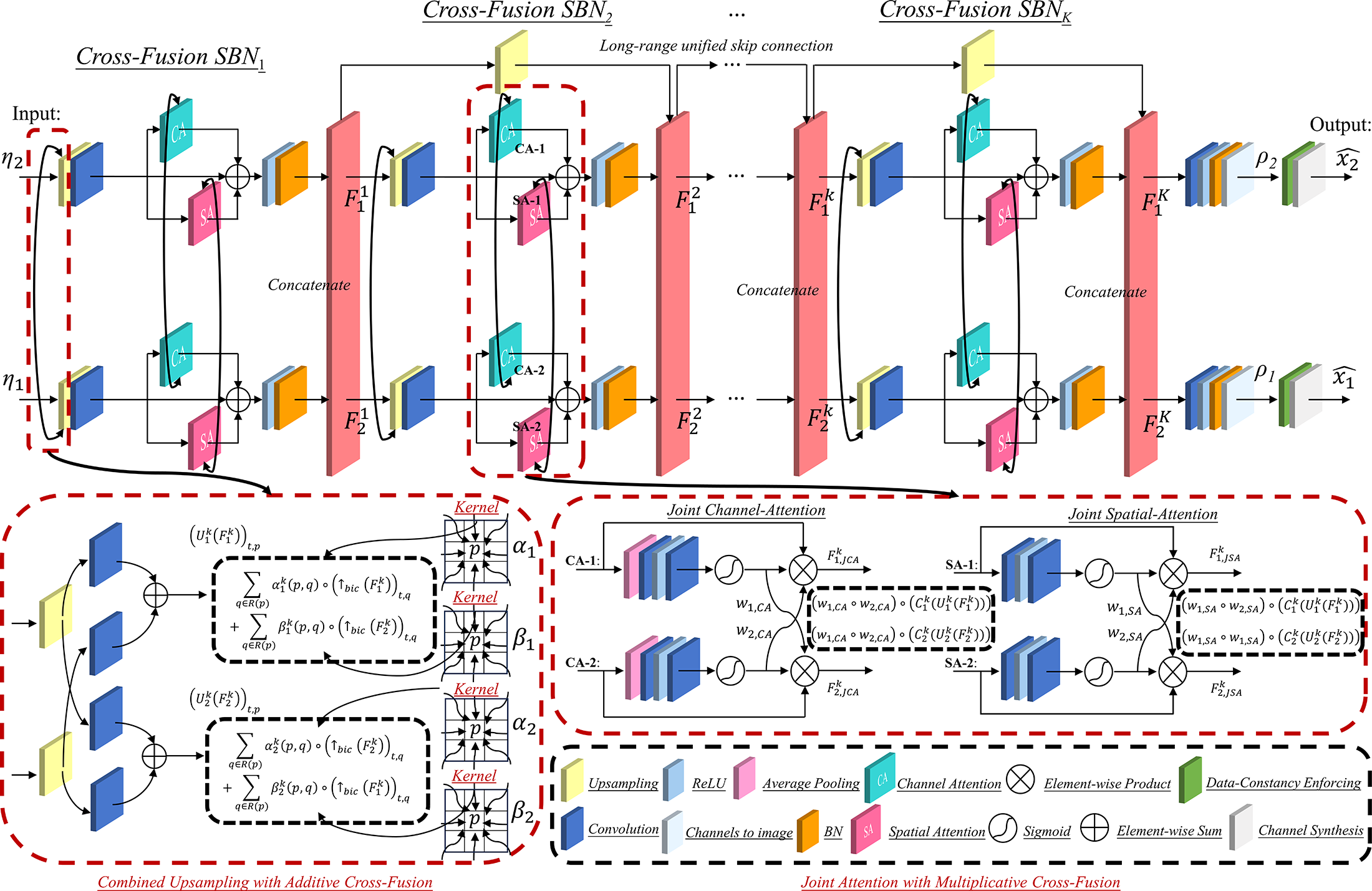
Figure 1: The two-stream PEARL architecture. The random variables $$$\eta_{1}\in\mathbb{R}^{1 \times {2} \times {w_{in}}\times {h_{in}}}$$$ and $$$\eta_{2}\in\mathbb{R}^{1 \times 2\times {w_{in}}\times {h_{in}}}$$$, along with $$$\rho_{1}\in\mathbb{R}^{1 \times {{2E} \times {w_{out}} \times {h_{out}}}}$$$ and $$$\rho_{2}\in\mathbb{R}^{1 \times {{2E} \times {w_{out}} \times {h_{out}}}}$$$, represent the network outputs. The final estimated images $$$\hat{x}_{i:i=1,2}$$$ are derived through data-consistency projection and channel synthesis.
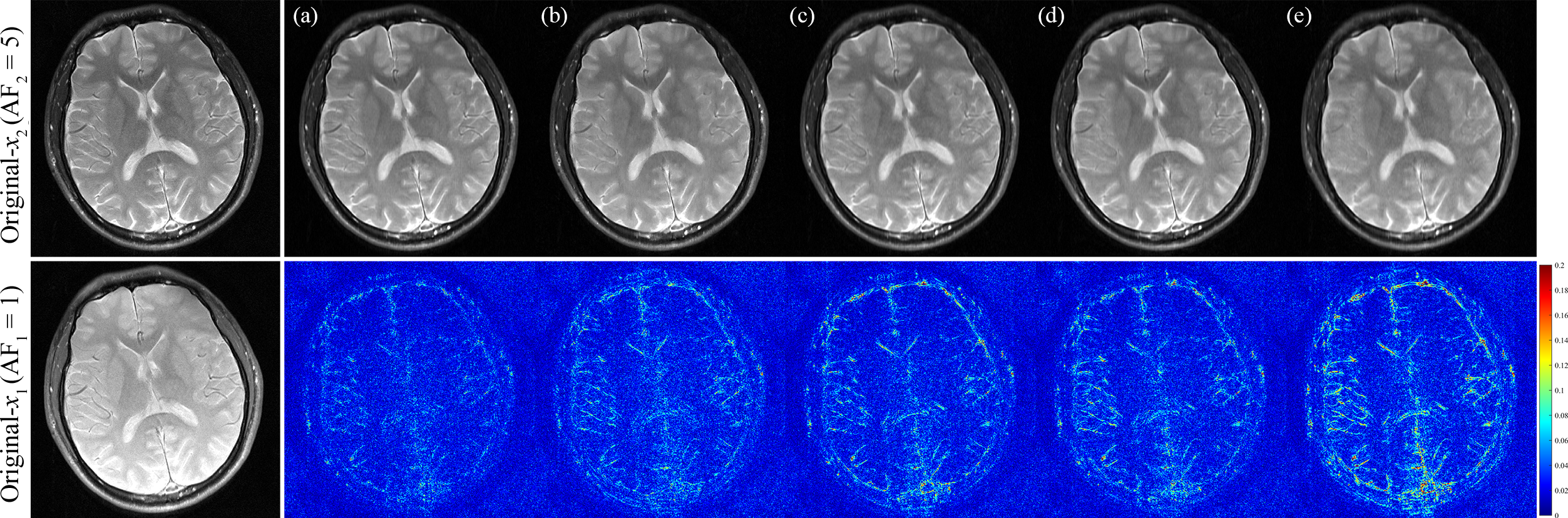
Figure 2: The Subject $$$\#1$$$ reconstruction at AF$$$_{1}$$$ = 1/AF$$$_{2}$$$ = 5. (a)-(e): PEARL, Joint-PICCS, Coupled DIP-TV, C$$$^{2}$$$onvDecoder, ConvDecoder-TV. The leftmost column displays the original images. Our approach exhibits superior performance, as evidenced by the error maps.
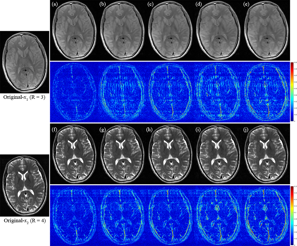
Figure 3: The Subject $$$\#2$$$ reconstruction at AF$$$_{1}$$$= 3/AF$$$_{2}$$$ = 4. (a)-(e)/(f)-(j): PEARL, Joint-PICCS, Coupled DIP-TV, C$$$^{2}$$$onvDecoder, ConvDecoder-TV. The leftmost column displays the original images. Our approach exhibits superior performance, as evidenced by the error maps.
DOI: https://doi.org/10.58530/2024/1768