1523
Deep Learning based de-noising and segmentation of Real-Time 3D Kinematic Imaging of the knee for modeling patellofemoral bone kinematics1Radiology, Stanford University, Stanford, CA, United States
Synopsis
Keywords: Functional/Dynamic, Visualization, kinematic, real-time
Motivation: Joint Maltracking or improper loading cannot be assessed with conventional, static MRI.
Goal(s): Demonstrate the feasibility of using images without motion to de-noise and segment real-time 4D images and generate 4D moving models.
Approach: In 31 subjects, a fully sampled image and many highly-undersampled images reconstructed from the same data acquired without motion are used to train a neural network to generate artifact-free images and bone segmentations for images acquired with motion.
Results: The resulting real-time images are recognizable however more work is needed to improve the reliability of the segmentation, especially in cases of large-scale or fast motion.
Impact: Deep learning based de-noising and segmentation of real-time 3D kinematic MR imaging make it possible to model knee kinematics and open the doors for the study of the knee in motion and under load for improved identification of pain generators.
Introduction
Musculoskeletal disorders are a leading source of pain, in part due to maltracking or improper loading of joints. Current kinematic MR imaging methods are largely limited to 2D acquisitions which is insufficient for imaging large and complex joints such as the knee.It is possible to reconstruct real-time 4D images of knee motion using DL methods to remove unwanted artifacts1,2. However, quantitative analysis of motion also requires bone segmentations for each frame. Manual segmentation of all timesteps is impractical. Current segmentation algorithms do not perform well on this data due to motion artifacts and unusual tissue contrast. In this work, we demonstrate the feasibility of using a DL network to both denoise and segment kinematic knee images as part of an end-to-end pipeline for real-time 4D analysis of kinematics.
Methods
31 subjects were scanned in a static position on a 3T whole-body scanner (GE SIGNA Premier) using a 16 channel receive-only phased-array flex coil, with at least one of the golden-angle reordered cones sequence (GA-Cones) protocols in Fig1 (46 acquisitions total).Our DL training, validation, and testing dataset was created using this data. Fully resampled images were reconstructed for DL-target images for denoising. Those images were manually segmented to be DL-targets for segmentation. Finally, 4D input images (SIs) were reconstructed from these same data with a (multiscale low-rank) MSLR algorithm1,3.
Data were divided by subject into training, validation, and test datasets (80%, 10%, 10%). We used a UNet architecture4 with an image-denoising pathway added before the final convolutional block, a learning rate of 1e-4 and batchsize of 32. Our loss function was the sum of mean absolute error of the output image (MAE), negative average dice scores (DSCs), and distance loss function (DLF)5. The input is three consecutive image slices. The output is a denoised image slice, and segmentations of patella, femur, and tibia. To avoid over-fitting, we implemented early stopping when the change in the total average validation DSC was less than 0.01 for 10 consecutive checkpoints (11 epochs of training).
4D images with motion (MIs) were analyzed using the 4-step pipeline outlined in Fig2:
Acquisition: Three subjects were scanned with the DESS protocol and one GA-Cones protocol during slow contraction of their quadriceps muscle and while repeatedly lifting their knee off the mat, at a rate of ~1Hz.
Reconstruction: MIs reconstructed with the MSLR algorithm1,3.
Denoising and Segmentation: The DL model generated bone segmentations of the MIs at every timestep. DESS images were manually segmented to generate high resolution reference 3D surface models.
Model Creation: Each frame of the MIs was analyzed as follows:
- Extracted the largest connected component for each DL-generated bone segmentation.
- Flood-filled each bone segmentation mask.
- Extracted bone surfaces using marching cubes.
- Rigidly registered DESS bone surfaces to the MI bone surfaces from (3).
Results
Fig3 shows representative denoised SIs and segmentations. Image quality for SIs is measured by MAE: 0.24, PSNR: 24.9 and SSIM: 0.86 (compared to MAE: 0.66, PSNR: 20.0, and SSIM: 0.578 for the MSLR images). Average DSCs are patella: 0.74, femur: 0.78, and tibia: 0.18. Fig4 shows representative denoised and segmented MIs. Fig5 shows a 4D model of a subject lifting their knee off the table.Discussion
The results demonstrate the feasibility of the end-to-end pipeline for 4D analysis of joint motion summarized in Fig2. The scale and type of motion are clearly visible in Fig5. The degradation of segmentation quality at 0.63s and 3s, especially in the patella, is likely due to motion distortions from large or rapid movement of the entire knee which can be reduced by changing the position of the participant and stabilizing the knee during joint motion.In Figs3&4 the tissue boundaries in the denoised images (B) are much clearer, demonstrating the network’s abilities to remove artifacts. However, the network struggles to differentiate between femur and tibia, likely due to the limited number of slices containing tibia in the training dataset, and often underestimates the patella (Fig3: 1-B and 2-B), or misidentifies fat as patella (Fig3: 3-B). These might be improved by adjusting the weight of the individual DSC values in the loss function. The table in Fig4 shows a disparity between the DSC calculated by slice and calculated by volume, implying that segmentations might be improved by including more image slices in the input.
Conclusion
This work showed a novel approach and feasibility of creating 4D models of whole knee motion from real-time kinematic knee MRI. These methods have the potential to provide novel insights into in vivo patellofemoral kinematics improving our understanding of mechanical factors of knee pain.Acknowledgements
This work was funded with research support from GE Healthcare and NIH R01AR07943.References
1. Hales L, Sandino C, Desai A, Chaudhari A, Kogan F. Three-Dimensional real-time dynamic knee MRI using 3D cones with a multiscale low-rank reconstruction. In: ISMRM Annual Meeting. ; 2022.
2. Hales Laurel, Desai A, Mazzoli V, Chaudhari A, Kogan F. De-noising of 4D real-time joint motion images using a convolutional neural network trained on static data. In: ISMRM. ; 2023.
3. Ong F, Zhu X, Cheng JY, et al. Extreme MRI: Large-scale volumetric dynamic imaging from continuous non-gated acquisitions. Magn Reson Med. 2020;84(4). doi:10.1002/mrm.28235
4. Buda M, Saha A, Mazurowski MA. Association of genomic subtypes of lower-grade gliomas with shape features automatically extracted by a deep learning algorithm. Comput Biol Med. 2019;109:218-225. doi:10.1016/j.compbiomed.2019.05.002
5. Caliva F, Iriondo C, Martinez AM, Majumdar S, Pedoia V. Distance Map Loss Penalty Term for Semantic Segmentation. Published online August 9, 2019. http://arxiv.org/abs/1908.03679
6. Fedorov A, Beichel R, Kalpathy-Cramer J, et al. 3D Slicer as an image computing platform for the Quantitative Imaging Network. Magn Reson Imaging. 2012;30(9):1323-1341. doi:10.1016/j.mri.2012.05.001
Figures
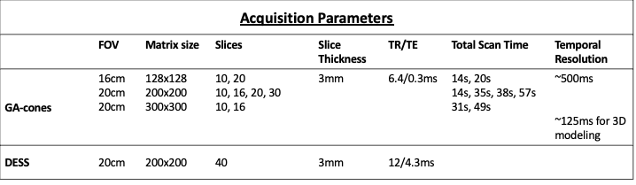
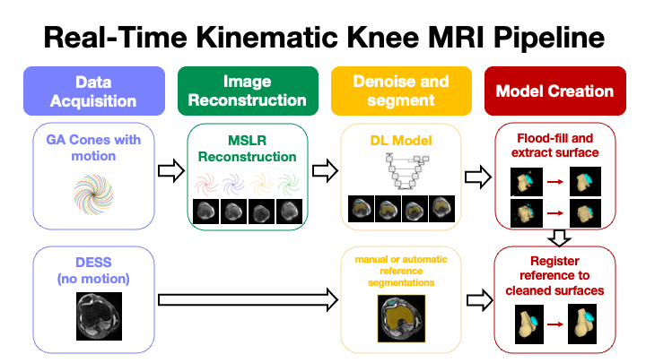
Figure 2: An illustration of the pipeline used to create 4D model of a moving knee for knee kinematics analysis.
Step 1: Acquire data with the GA-Cones protocol and DESS.
Step 2: MSLR reconstruction of the GA-Cones data.
Step 3: DL dynamic segmentations and denoising of the cones images and segmentation of DESS.
Step 4: Clean the dynamic segmentations and register the DESS segmentation of each bone to the corresponding cleaned dynamic surface.
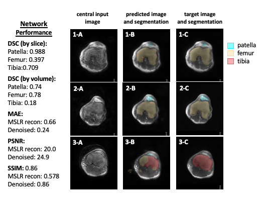
Figure 3: Representative examples of network's performance in SIs. A: central input image, B: the generated denoised image and segmentation overlay. C: the fully sampled target image and manual segmentation. In all three cases the network struggles to differentiate between tibia and femur. This is worst in panel 3-B where there is no femur. The network also underestimates patella size (1-B, 2-B), and sometimes misidentifies fat as patella (3-B). The table shows quantitative measures of the network performance.
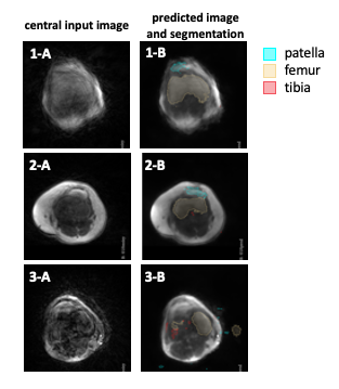
Figure 4: Representative examples of the DL network's performance on MIs. Column A shows the central input image, and Column B the denoised input image with the generated segmentation overlayed.
These segmentations have less well-defined edges than the segmentations generated for SIs. This is possibly due to distortion due to bulk motion. Note that the patella, has more distortion from motion artifacts then the femur which is in the middle of the knee.
There are no quantitative measures of image quality for MIs because there is not target image.
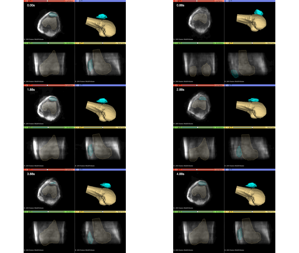
Figure 5: Each pane of the gif shows a different view of the knee as the participant lifts their knee off the table. The top right pane shows the 3D model.
The femoral motion is reasonable, throughout the motion, but the patellar motion is still unreliable at the points of greatest motion (0.63 and 3.00s). The animation was generated using 3D Slicer 6