Introduction

MR-based depiction of bony tissue is increasingly being investigated as a radiation-free alternative to computed tomography for various diagnostic questions. However, to reach adequate image quality, lengthy exams are typically still required. In this work, we implemented and tested a deep learning driven strategy to shorten the overall acquisition time in IR-prepared ultra-short echo time (UTE) MR imaging.

Methods

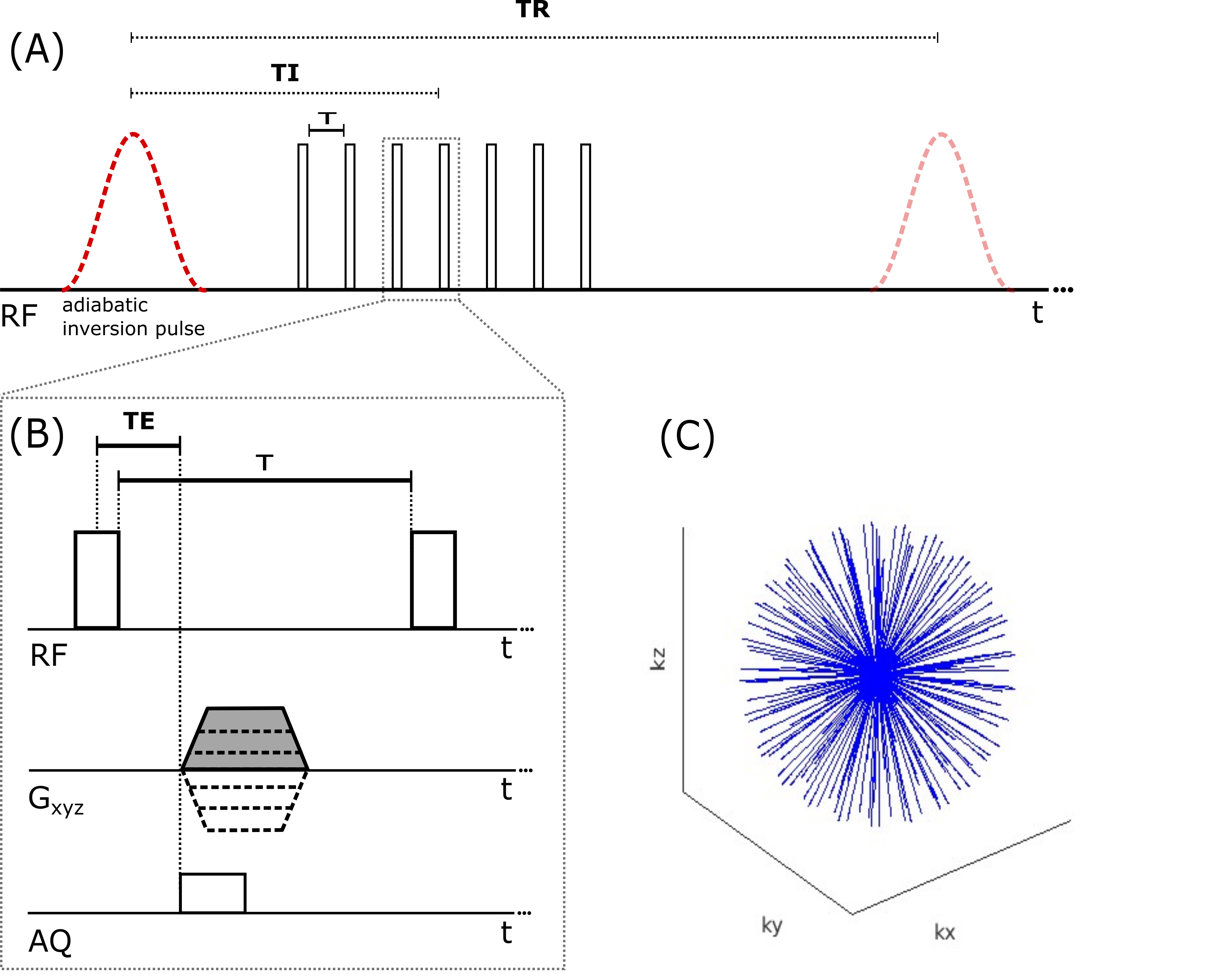
An IR-prepared UTE sequence similar to [1] was implemented in Pulseq [2] (see Fig. 1). Data sampling was performed using ramp sampling and a 3D radial trajectory, equally distributed on the k-space sphere (a.k.a koosh ball). Using a long adiabatic inversion pulse, this approach suppresses the signal of tissues with longer T2 relaxation times, thereby enabling a robust differentiation of compartments of cortical and trabecular bone with short T2*. For each adiabatic IR pulse, seven projections centered around TI = 64$$$\ $$$ms were recorded with a temporal spacing of τ = 4.1$$$\,$$$ms between each. The adiabatic IR pulse had the shape of a hyperbolic secant with a duration of 10$$$\,$$$ms centered around -220 Hz, which corresponds to the midpoint between fat and water at 3$$$\,$$$T. k_max corresponded to an isotropic spatial resolution of 1.6$$$\,$$$mm. Sample data were acquired in the left ankle of one healthy volunteer and the head of another at 3$$$\,$$$T field strength (Siemens Magnetom Prisma). Benchmark data consisting of 56$$$\,$$$k projections, as well as prospectively undersampled data with 21$$$\,$$$k projections were acquired in 20:00$$$\,$$$min (ankle) and 7:30$$$\,$$$min (head) scan time. The corresponding minimum FOV (corresponding to largest gap in k-space until k_max) was 21$$$\,$$$cm for 56$$$\,$$$k projections and 13$$$\,$$$cm for 21$$$\,$$$k projections. From the fully sampled dataset (ankle), undersampled versions were simulated by retrospectively removing projections to build sets with 28$$$\,$$$k and 11.2$$$\,$$$k respectively. Higher acceleration was also simulated in the head dataset by using only half of the acquired data (10.5$$$\,$$$k projections).
To enable the reconstruction of undersampled and thus accelerated scans, a thresholded Landweber styled algorithm was implemented which features the enforcement of the physical measurement model (acquired data $$$y$$$, coil sensitivities), the sparsity in image space (minimization of L1-norm) as well as the integration of a pre-trained denoising convolutional neural network (DnCNN,[3]). In the current version of the algorithm, we used an “off-the-shelf” DnCNN model provided by MathWorks, not specifically trained for bone MRI.

Pseudo-code:

Input: $$$x_{0} = A^{*}y, \gamma = 1, P_{0}=angle(x_{0})$$$
for $$$m=1,2,...,n$$$
$$$\,\,\,\,\,\,\,\,$$$$$$x_{m}=x_{m-1}-\gamma A^{*}(Ax_{m-1}-y)$$$
$$$\,\,\,\,\,\,\,\,$$$$$$x_{m}=real(x_{m}\circ e^{i\cdot(-P_{m-1})})$$$
$$$\,\,\,\,\,\,\,\,$$$$$$x_{m}=DnCNN(x_{m})$$$
$$$\,\,\,\,\,\,\,\,$$$$$$x_{m}=x_{m}\circ e^{i\cdot P_{m-1}}$$$
$$$\,\,\,\,\,\,\,\,$$$$$$x_{m}=STH_{\sigma}(x_{m})$$$
$$$\,\,\,\,\,\,\,\,$$$$$$P_{m}=angle(x_{m})$$$
end
return $$$x_{n}$$$

Matrix $$$A$$$ represents the MRI operator including a 3D gridding procedure [4], initialized with the trajectory information and the coil sensitivities, which were estimated from the densely sampled central part of the 3D k-space using ESPIRIT [5]. $$$x_{0}$$$ was determined by a “naïve reconstruction” using a grid size of 256 x 256 x 256. $$$STH_{\sigma}$$$ applies a soft threshold in image space with a threshold of $$$\sigma$$$, which was determined empirically based on the noise level. A number of $$$n$$$ = 15 was chosen for the reconstruction of the ankle dataset, and $$$n$$$ = 13 for the head dataset. In the following, we refer to the proposed method as S3MOB (Speedy 3D MRI Of Bone). For comparison, conjugate gradient SENSE [6] was applied to the same datasets.

Results

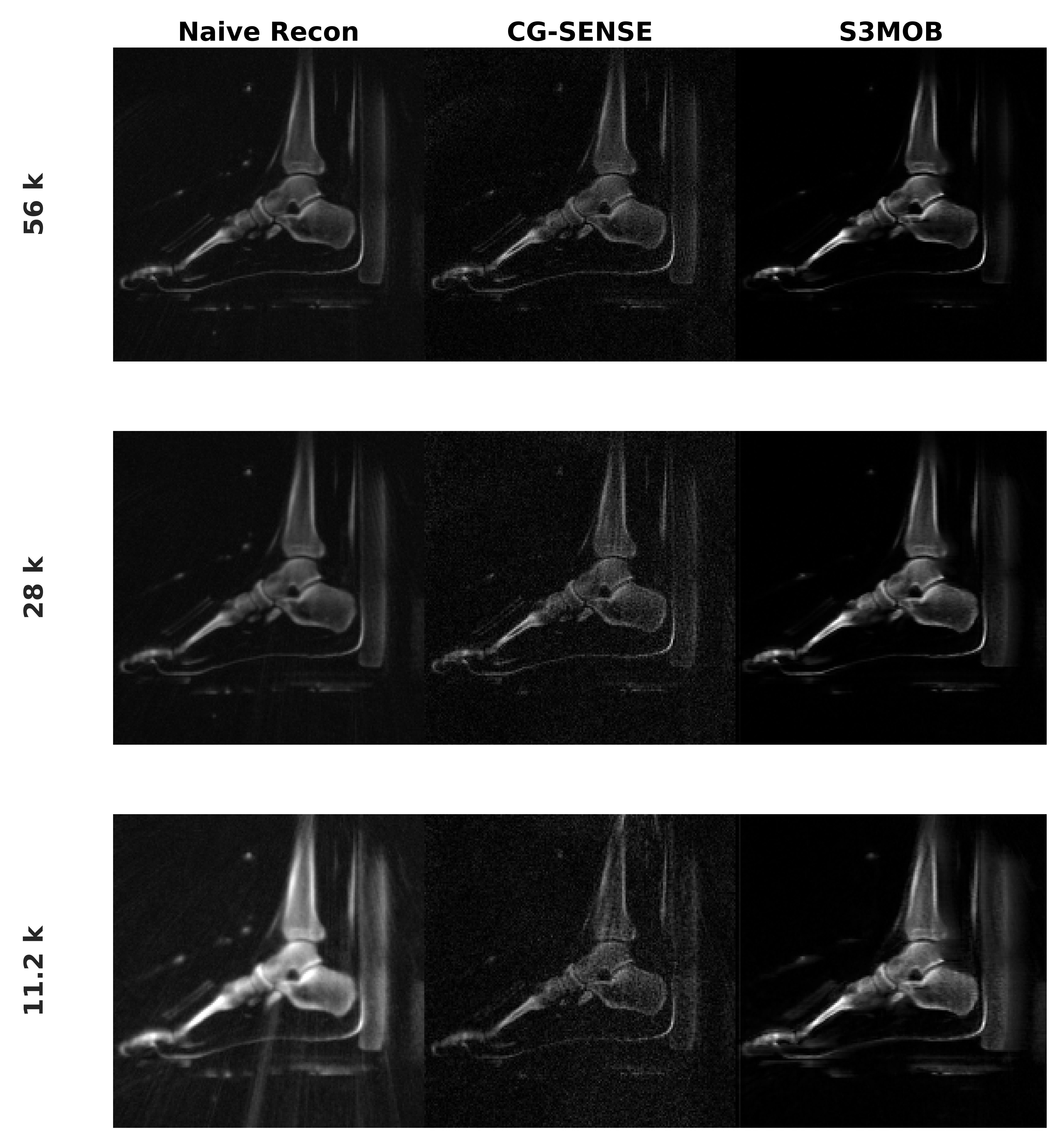
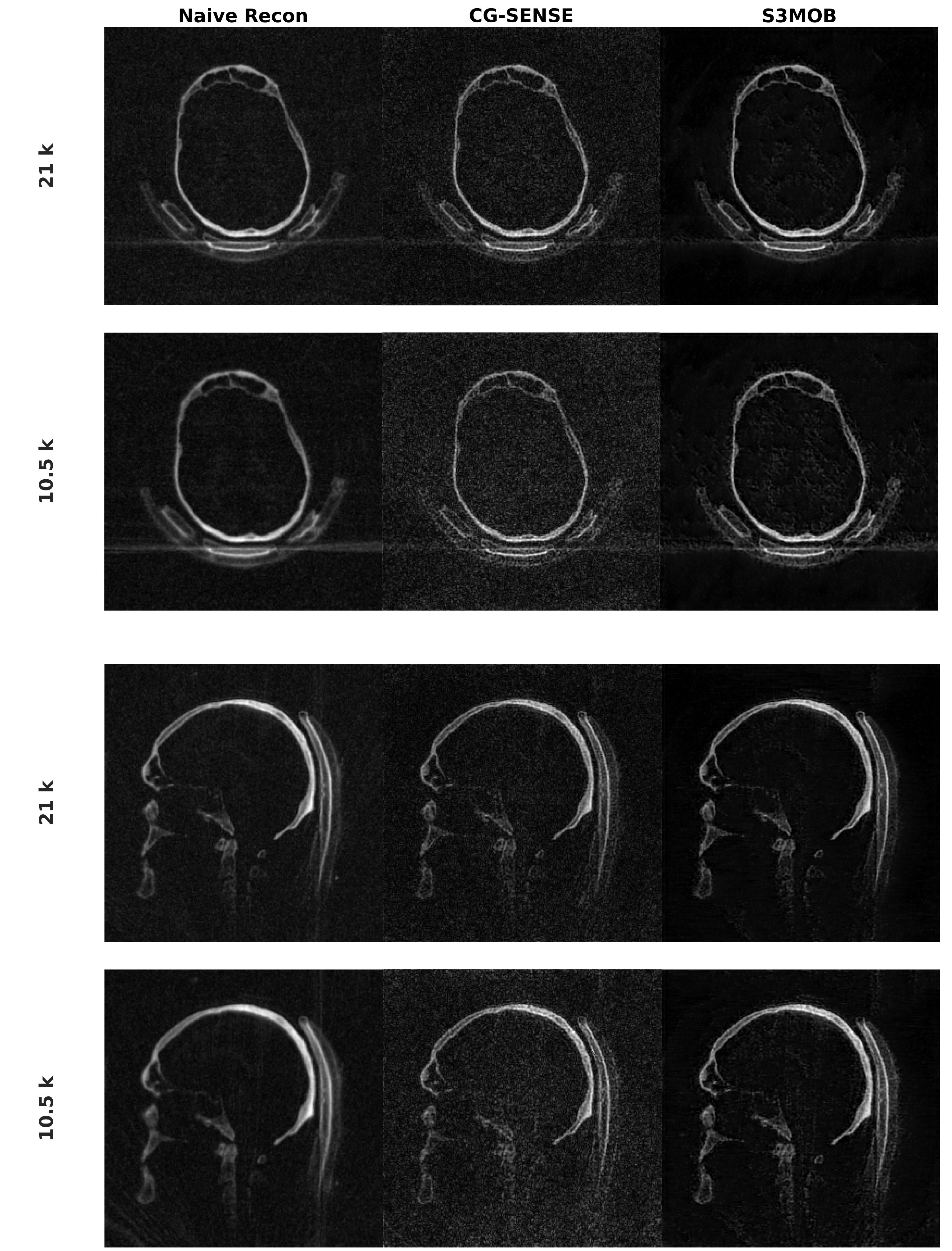
Fig. 2 and Fig. 3 depict the reconstructions of ankle and head data for naïve gridding reconstruction, iterative SENSE, and the proposed S3MOB method with different numbers of acquired projections. With 56$$$\,$$$k projections, the naïve reconstruction results in a depiction of the ankle with low artifact level, good SNR and sharp edges (Fig. 2). Since the data is not fully sampled in the periphery of k-space, iterative SENSE could increase sharpness slightly, however at the cost of also increasing noise. This effect is more pronounced for higher acceleration factors. The application of S3MOB resulted in a good compromise between sharpness, SNR and artifact level. This is confirmed by the head data shown in Fig. 3. Bone microstructure could be resolved with good SNR, even with only 10.5$$$\,$$$k projections, corresponding to an acquisition time of 3:45$$$\,$$$min. Using an NVIDIA RTX A6000 GPU (48$$$\,$$$GB), the reconstruction time for S3MOB was between one (10.5$$$\,$$$k projections) and seven minutes (56$$$\,$$$k projections) for the presented examples.

Discussion & Conclusion

The proposed data-driven S3MOB technique represents a promising method to accelerate MRI in bony tissues. Next steps include training the denoising CNN specifically for the imaging task, studying the impact of the acceleration on quantitative imaging (T2*- or proton density mapping) as well as the combination with alternative means of acceleration, e.g. exploiting more efficient trajectories like FLORET [7].

Acknowledgements

Presented work was partially funded by the Interdisciplinary Center for Clinical Research in Würzburg under Research Grant F-437.