Introduction

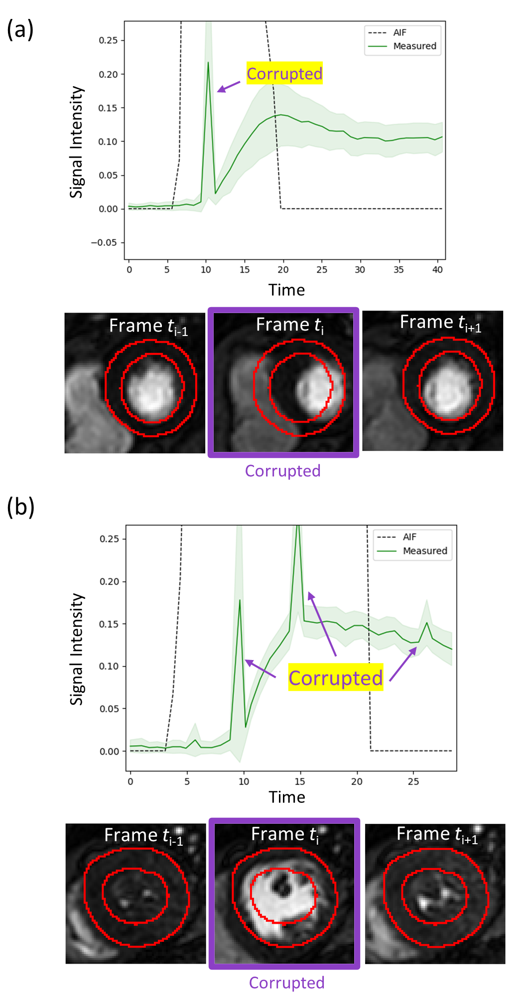
Pixel-wise myocardial perfusion quantification offers higher spatial resolution, enabling the detection of small perfusion defects that may go unnoticed in segment-wise quantification. While many studies have explored robust pixel-wise myocardial blood flow quantification^1,2,3,4, further investigation is needed to accurately measure the delay time between the arterial and myocardial tissue tracer arrival. In healthy hearts, minimal and consistent delays over heart segments signify normal perfusion, while ischemic hearts exhibit increased and variable delays, indicating impaired blood flow⁵. Estimating the delay is however challenging because, in addition to its sensitivity to noise, cardiac or respiratory motion can lead to artifacts that have a strong impact on the delay estimation (Figure 1). Here we propose a DL-based approach that identifies these motion artifacts as outliers along the time curve of each voxel and removes them from the perfusion quantification. This ensures accurate perfusion quantification even in cases of residual motion. The proposed approach only requires simulated data for training and can then be applied to in-vivo data.

Methods

Fermi Model: The pixel-wise signal intensity $$$c(t)\equiv\;c(t,x)$$$ at time $$$t$$$ and location $$$x$$$ is modeled as the time-convolution of the arterial input function $$$c_{\mathrm{AIF}}(t)$$$ with the Fermi function⁶ $$$r_{\mathrm{F}}(t,F,\tau,k)$$$, dependent on pixel-wise flow $$$F\equiv\;F(x)$$$, delay $$$\tau\equiv\;\tau(x)$$$, and decay $$$k\equiv\;k(x)$$$, as following-
$$c(t)=c^{\mathrm{Invivo}}_{\mathrm{AIF}}(t)\ast\;r_{\mathrm{F}}(t,F,\tau,k)=\int_{0}^{t}r_{\mathrm{F}}(t,F,\tau,k)c_{\mathrm{AIF}}(t-t^{\prime})dt^{\prime},\tag{1}\label{forward}$$
where $$$r_{\mathrm{F}}(t,F,\tau,k)=\frac{F}{1+\mathrm{exp}\left((t-\tau)k\right)}H(t-\tau)$$$ depicting the Heavy-side function.

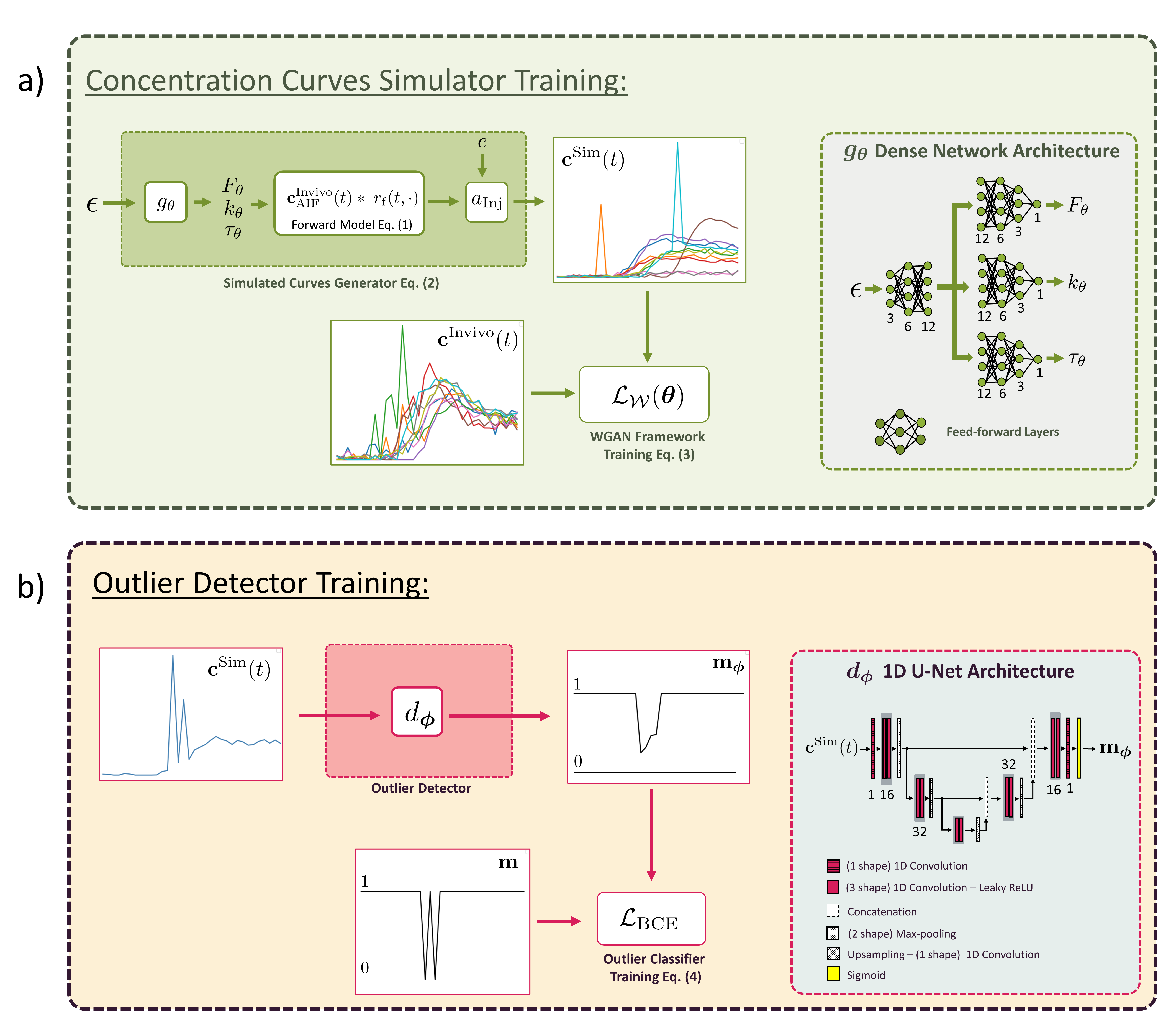
Simulator Training (Figure 2a): A generator $$$g_{\theta}(\epsilon)$$$ is applied to standard-Gaussian noise $$$\epsilon$$$ to synthesize $$$F_{\theta},\tau_{\theta},$$$ and $$$k_{\theta}$$$, followed by applying the forward model $$$\eqref{forward}$$$, and adding Rician noise $$$e$$$ and outliers to simulate signal intensities $$$c^{\mathrm{Sim}}(t)$$$ as shown-

$$c^{\mathrm{Sim}}(t)\equiv\;c^{\mathrm{Sim}}(t;\epsilon,\theta)=a_{\mathrm{Inj}}\left(\left(c^{\mathrm{Invivo}}_{\mathrm{AIF}}(t)\ast\;r_{\mathrm{F}}(t,F_{\theta},\tau_{\theta},k_{\theta};\epsilon)\right)+e\right),\tag{2}\label{sim_gen}$$

where $$$a_{\mathrm{Inj}}$$$ denotes the injection of outliers, and $$$[F_{\theta},\tau_{\theta},k_{\theta}]=g_{\theta}(\epsilon)$$$. Let $$$\mathbf{c}^{\mathrm{Sim}}=[c^{\mathrm{Sim}}(t_{0}),\ldots,c^{\mathrm{Sim}}(t_{N_{T}})]\in\mathbb{R}^{N_{T}}$$$ be a signal vector where $$$N_{T}$$$ is the number of measurement time-points. The outliers that $$$a_{\mathrm{Inj}}$$$ introduces at random $$$\mathbf{c}^{\mathrm{Sim}}$$$ time-component(s) is modeled as 3 to 5 times the standard-deviation of $$$\mathbf{c}^{\mathrm{Sim}}$$$. Hereafter, we employ the Wasserstein generative adversarial framework^7,8 (WGAN) to learn $$$\mathbf{c}^{\mathrm{Sim}}$$$ such that its distribution approximates that of the invivo intensities $$$\mathbf{c}^{\mathrm{Invivo}}\in\mathbb{R}^{N_{T}}$$$ with respect to the Wasserstein-1 metric $$$\mathcal{W}$$$ by minimizing the following-

$$\mathcal{L}_{\mathcal{W}}(\boldsymbol{\theta})=\underset{\boldsymbol{\theta}}{\min}\;\mathcal{W}\left(\mathbf{c}^{\mathrm{Sim}}(\boldsymbol{\theta}),\mathbf{c}^{\mathrm{Invivo}}\right)\tag{3}\label{wgan}$$

Detector Training (Figure 2b): Outliers are simulated through $$$a_{\mathrm{Inj}}$$$, allowing us to construct a label vector $$$\mathbf{m\in\mathbb{R}^{N_{T}}}$$$ whose components are zero if their location corresponds to an outlier or one otherwise. We train a detector network $$$d_{\boldsymbol{\phi}}$$$ to identify outliers in $$$\mathbf{c}^{\mathrm{Sim}}$$$ using the binary cross-entropy (BCE) loss⁹ as shown-
$$\mathcal{L}_{\mathrm{BCE}}(\boldsymbol{\phi})=\underset{\phi}{\min} \; \mathrm{BCE}( \mathbf{m}, d_{\boldsymbol{\phi}}\left(\mathbf{c}^{\mathrm{Sim}}\right)),\tag{4}\label{bce}$$
where $$$\mathbf{c}^{\mathrm{Sim}}$$$ are generated through \eqref{sim_gen} by sampling $$$\epsilon$$$, after training $$$g_{\theta}$$$ with \eqref{wgan}.

Parameter Inference: We apply $$$d_{\boldsymbol{\phi}}$$$ to $$$\mathbf{c}^{\mathrm{Invivo}}$$$, and pass the result through $$$H$$$, ensuring that the output is one when $$$\mathbf{m}_{\boldsymbol{\phi}}=d_{\boldsymbol{\phi}}(\mathbf{c}^{\mathrm{Invivo}}(t))$$$ is greater than $$$p$$$, which we set to $$$0.2$$$, and zero otherwise. This yields our predicted mask $$$\mathbf{m}_{\mathrm{pred}}=H\left(\mathbf{m}_{\boldsymbol{\phi}}-p\right)$$$ which we use to detect and mask outliers before LBFGS curve-fitting, resulting in our proposed LBFGS-OD approach.
$$F_{\mathrm{pred}},\tau_{\mathrm{pred}},k_{\mathrm{pred}}=\omega_{\mathrm{LBFGS}}(\mathbf{m}_{\mathrm{pred}}\cdot\;\mathbf{c}^{\mathrm{Invivo}}),$$
where $$$\omega_{\mathrm{LBFGS}}$$$ denotes fermi-deconvolution⁶ using an LBFGS¹⁰ algorithm.

Results and Discussion

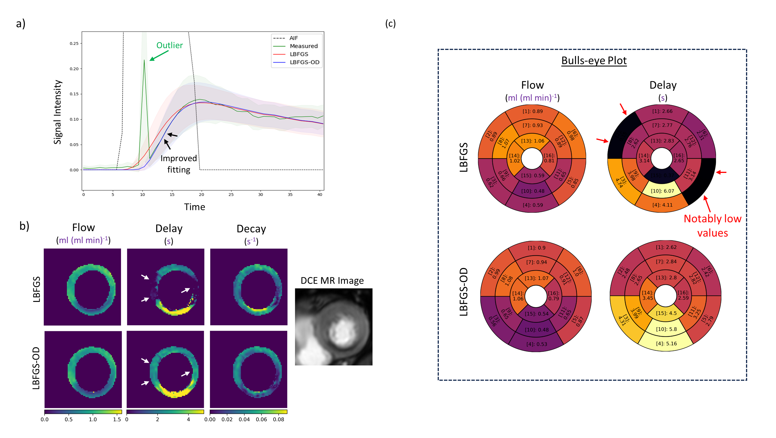
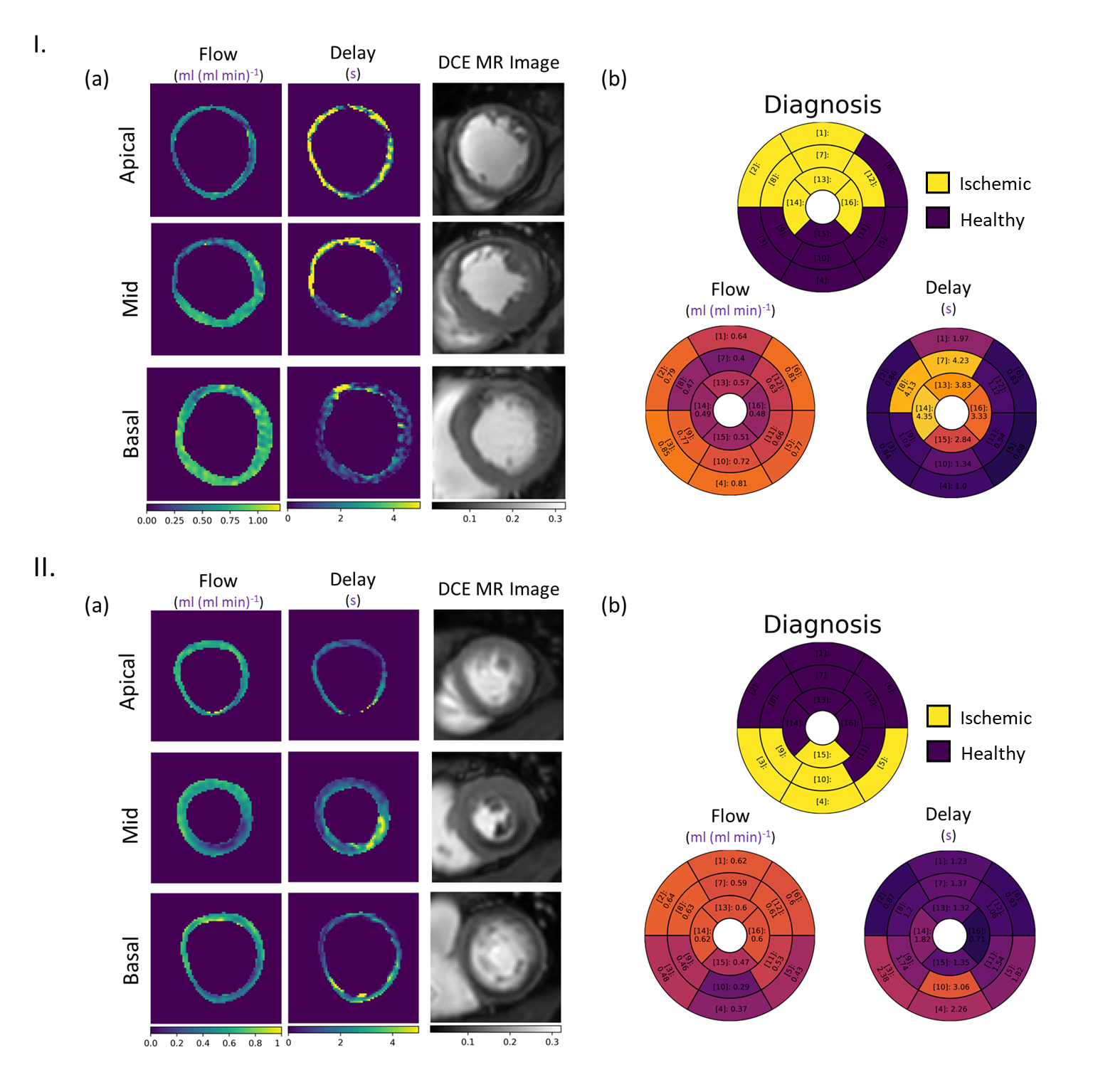
In Figure 3a, we compare the results of LBFGS with our proposed LBFGS-OD. We observe that LBFGS-OD effectively masks the outlier occuring during the rise time of the signal (black arrows) crucial for precise delay estimation. Figure 3b provides further evidence that LBFGS-OD preserves delay estimates in the outlier-affected area (white arrows). In contrast, LBFGS underperforms in such regions which causes the delay estimates of the segment-wise AHA¹¹ bulls-eye plot analysis as shown in Figure 3c to be significantly lower in specific segments indicated by the red arrows, a pattern not observed in the case of LBFGS-OD.

In Figure 4, we showcase the estimation performance of LBFGS-OD both at pixel and segment level for two patients. For both patients, the flow and delay bulls-eye plot show good agreement with the clinical diagnosis.

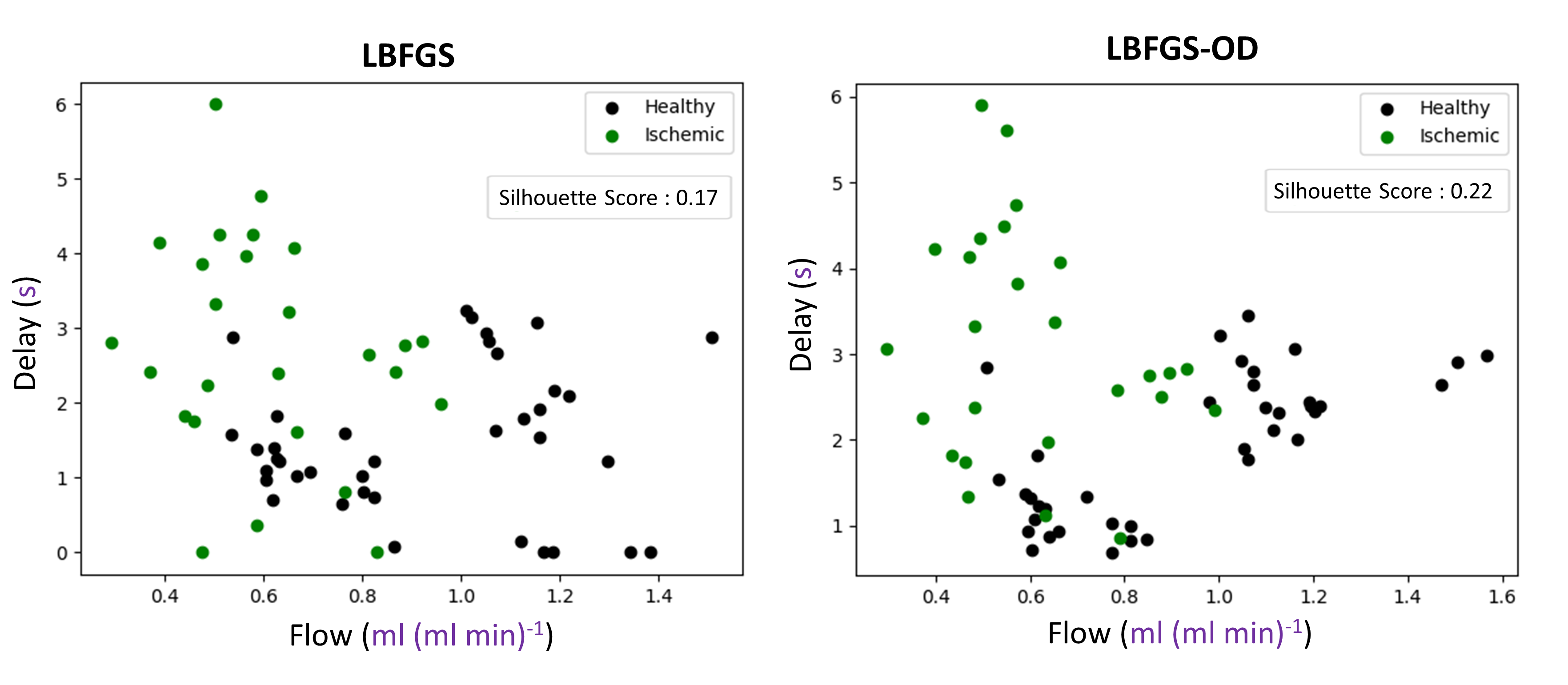
Figure 5 depicts a flow-vs-delay analysis on 26 ischemic and 38 healthy segments from four patients, totaling 64 segments. An examination of the graph shows that LBFGS-OD enhances the differentiation between healthy and ischemic segments compared to LBFGS. The higher Silhouette Score¹² provides quantitative evidence of improved cluster separation with LBFGS-OD. This underscores the significance of incorporating both delay and flow for enhanced diagnostic capabilities in detecting perfusion defects.

Conclusion

We successfully demonstrated the application of deep learning for detecting outliers in invivo myocardial perfusion data, where prior knowledge of the specific outlier locations is not available in real scenarios. We achieved this by training our network solely on simulated data, generated by another network that closely mimics invivo data. Additionally, our results indicate that the removal of outliers improves the estimation of the perfusion delay parameter, which holds valuable diagnostic insights.

Acknowledgements

This work was supported by the German Research Foundation, project number GRK2260, BIOQIC.