Introduction

Cardiac $$$T_1$$$ mapping is a powerful MRI technique for identifying the tissue structure and underlying pathological causes of the myocardium. Extracellular volume (ECV) fraction, a quantitative metric that can be derived from pre- and post-contrast $$$T_1$$$values, is an emerging biomarker for amyloidosis¹, myocardial injury², and particularly diffuse fibrosis^{3, 4}, which is known to be challenging to detect using the conventional late gadolinium enhancement (LGE) method. Cardiac ECV mapping is challenging due to respiratory and cardiac motions. Also, $$$T_1$$$ values change over time after the administration of contrast agent injection, which makes it difficult to estimate the post-contrast $$$T_1$$$ accurately for the relatively long 3D acquisition. As a result, the existing methods are limited to 2D ECV mapping, which often suffers from limited spatial coverage and/or through-plane resolution⁵. In this work, we propose a new method to enable free-breathing, 3D ECV mapping of the whole heart.

Method

Data acquisition
All experiments were performed under a study protocol approved by our local institutional review board (IRB). Four healthy volunteers (1M and 3F; 43 ± 16 years) were imaged using a 3T PET/MR scanner (Biograph mMR, Siemens Healthcare, Erlangen, Germany). Imaging was performed using a free-breathing, ECG-gated, inversion recovery (IR) sequence with sparse-sampling (Fig.1) ⁶, before and after the contrast-agent injection (Dotarem®, 0.1 mmol/kg). Data was acquired using a 3D spoiled gradient-echo (SPGR) readout with the following imaging parameters: field-of-view (FOV) = 308×308×144 mm3, spatial resolution = 1.9×1.9×4.5 mm3, flip angle (FA) = 9°, TR = 4.2 ms, TE = 1.7 ms, 10-(3)-10-(3) protocol, acquisition window per frame = 138.6 ms, and total number of frames = 900 (which corresponds to acquisition times of 12.4 ± 1.4 and 11.0 ± 0.7 min for pre- and post-contrast injection acquisitions, respectively).
Reconstruction
Dynamic MR images were reconstructed using the Linear Tangent Subspace Alignment (LTSA) model^7,8, which exploits the low-dimensional manifold structure of dynamic MR images in order to reduce the dimensionality of the image reconstruction problem. The LTSA model expresses dynamic MR images $$$X \in \mathbb{C}^{M\times N}$$$ where $$$M$$$ is the number of pixels and $$$N$$$ the number of time frames, split into $$$C$$$ neighborhoods $$$X_c$$$, $$$c=1,\dots,C$$$ as: $$$X_c = \boldsymbol{T} \boldsymbol{L}_c \boldsymbol{\Phi}_c^\top$$$, where $$$\boldsymbol{T}$$$ represents the global coordinates of the manifold, $$$\boldsymbol{L}_c$$$ is a linear alignment transform from local to global coordinates and $$$\boldsymbol{\Phi}_c$$$ is a set of temporal bases estimated from the acquired training lines via SVD. Neighborhoods were selected to match respiratory phases, which were estimated using a navigator acquired near the liver/lung interface. The resulting reconstruction problem was: $$\arg\min_{T,L} \left\|\boldsymbol{\Omega}\left( \boldsymbol{F}_s \sum_c \boldsymbol{T} \boldsymbol{L_c} \boldsymbol{\Phi_c} \boldsymbol{\Pi_c}\right) - \boldsymbol{s} \right\|_2^2 + \frac{\mu_L}{2} \left\|\boldsymbol{L}\right\|_F^2 + \frac{\mu_T}{2} \left\|\boldsymbol{T}\right\|_F^2 + \lambda_T \left\|\mathcal{D}\boldsymbol{T}\right\|_1 + \lambda_L \left\|\boldsymbol{L}\right\|_1,$$ where $$$\boldsymbol{\Omega}$$$ is the sparse sampling operator, $$$\boldsymbol{F}_s$$$ is the nonuniform Fourier transform operator implemented via NUFFT⁹, $$$\boldsymbol{\Pi_c}$$$ is a frame selection operator, $$$\boldsymbol{s}$$$ is the acquired k-space data, $$$\mu_L$$$ and $$$\mu_T$$$ are scalar weights controlling the $$$\ell_2$$$ regularization strength on $$$\boldsymbol{T}$$$ and $$$\boldsymbol{L}$$$ respectively, $$$\left\|.\right\|_F$$$ is the Frobenius norm, $$$\mathcal{D}$$$ is the finite difference operator and $$$\lambda_T$$$ and $$$\lambda_L$$$ are scalar weights controlling the strength of the total variation on $$$\boldsymbol{T}$$$ and sparsity penalty on $$$\boldsymbol{L}$$$ respectively. The alternating direction method of multipliers¹⁰ was used to solve this optimization problem.
T₁ mapping
Joint $$$T_1$$$ and transmit $$$B_1$$$ ($$$B_1^+$$$) mapping was performed as in ⁶, using a grid search over a dictionary of basis functions generated following Bloch equations for a range of $$$T_1$$$ and effective $$$B_1^+$$$ values. For each pixel and each respiratory bin, a grid search was performed over the parameters, following the variable projection method. For mapping of the post-contrast images, basis functions were generated assuming a linear $$$T_1$$$ change over time, thus adding a third parameter, the $$$T_1$$$ rate of change, to the grid search. We compared the proposed method with Modified Look-Locker Inversion Recovery (MOLLI).

Results

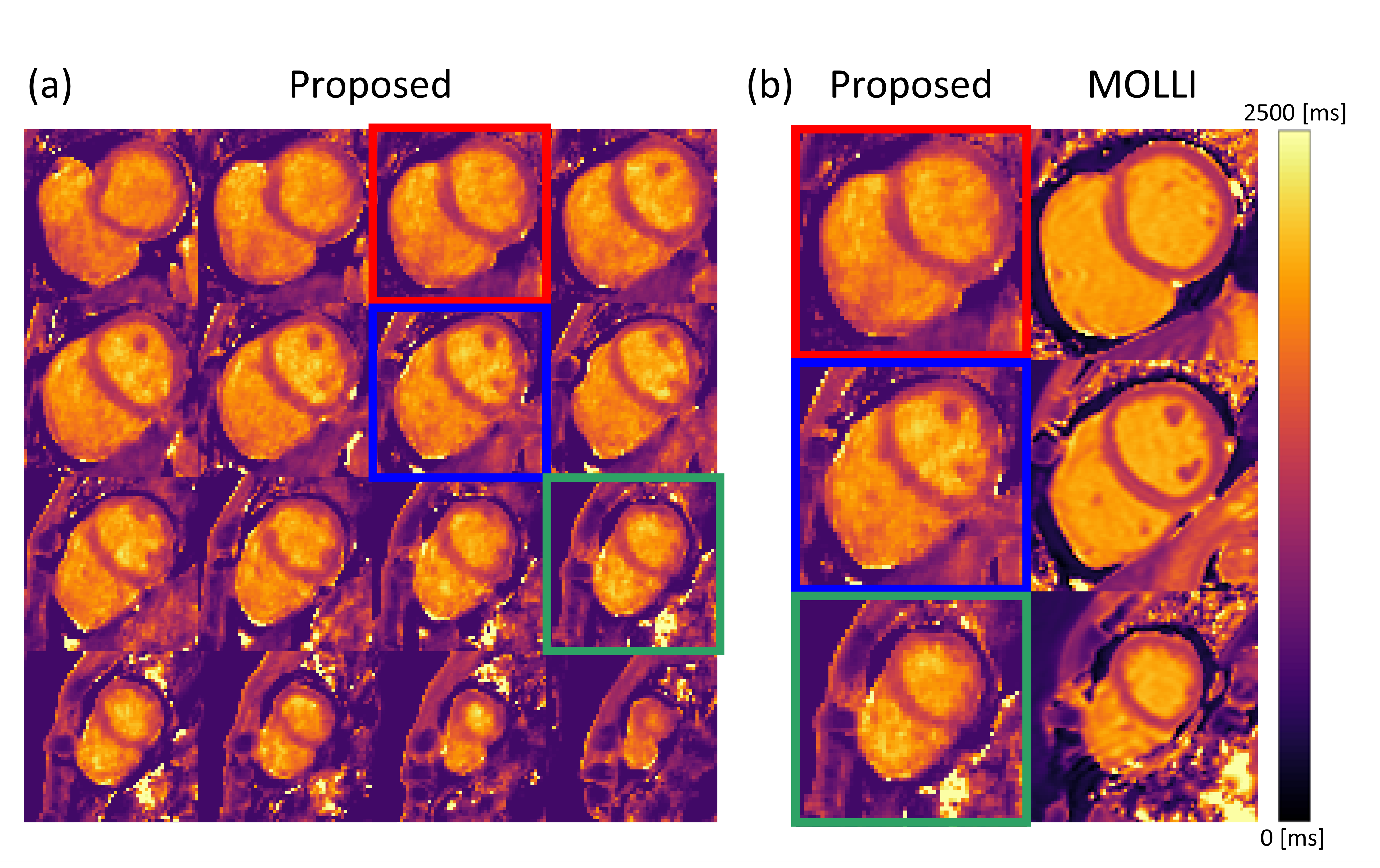
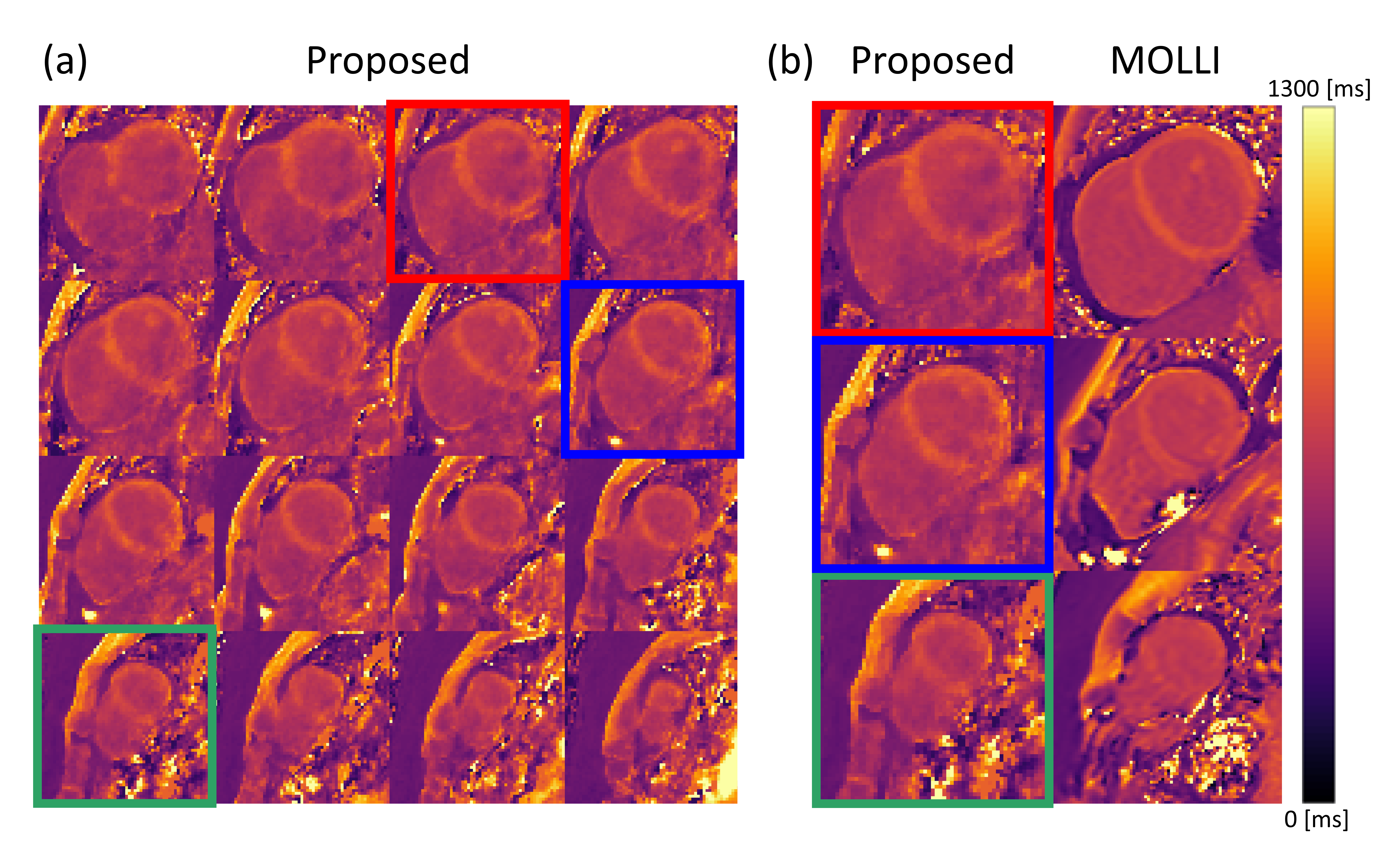
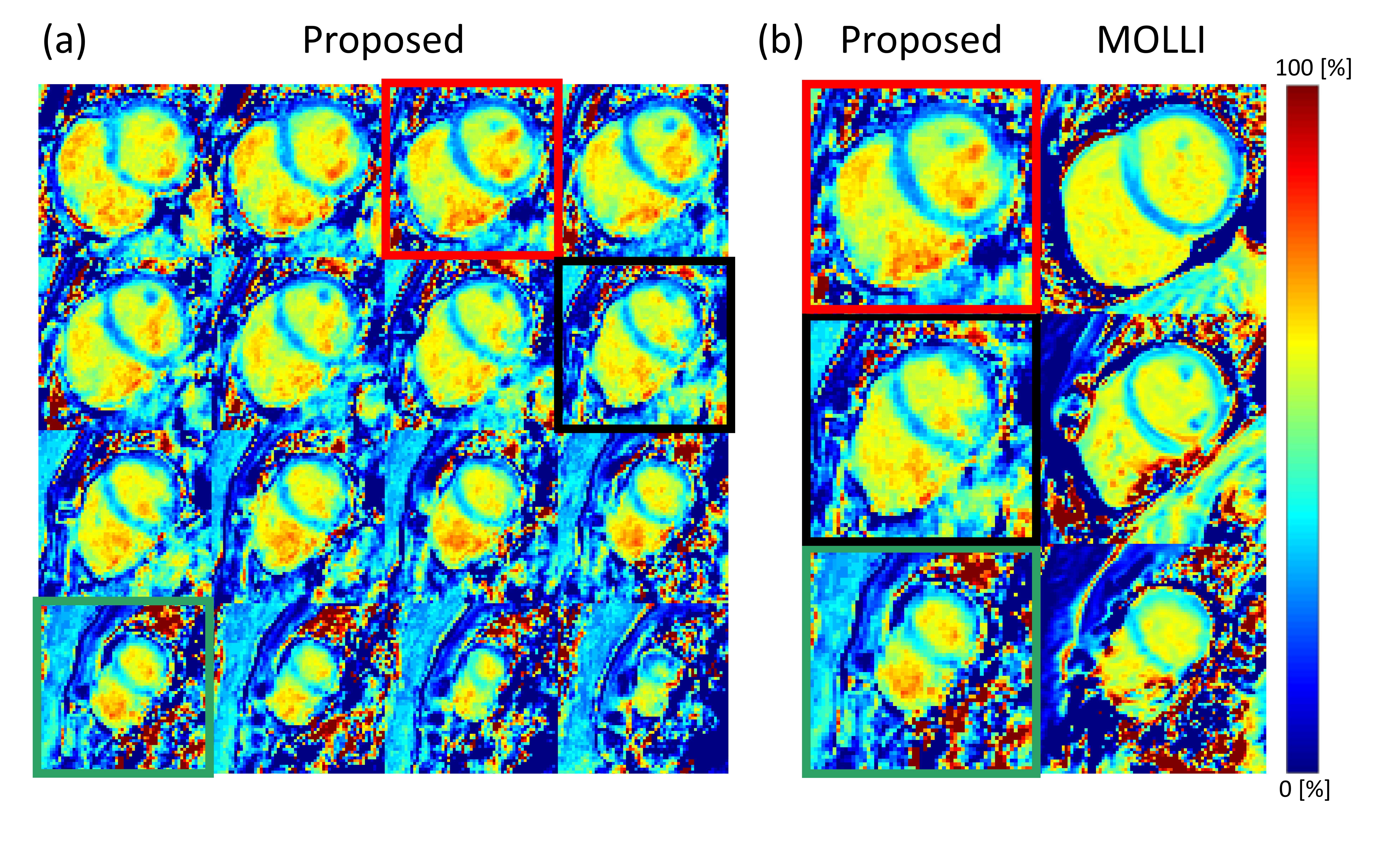
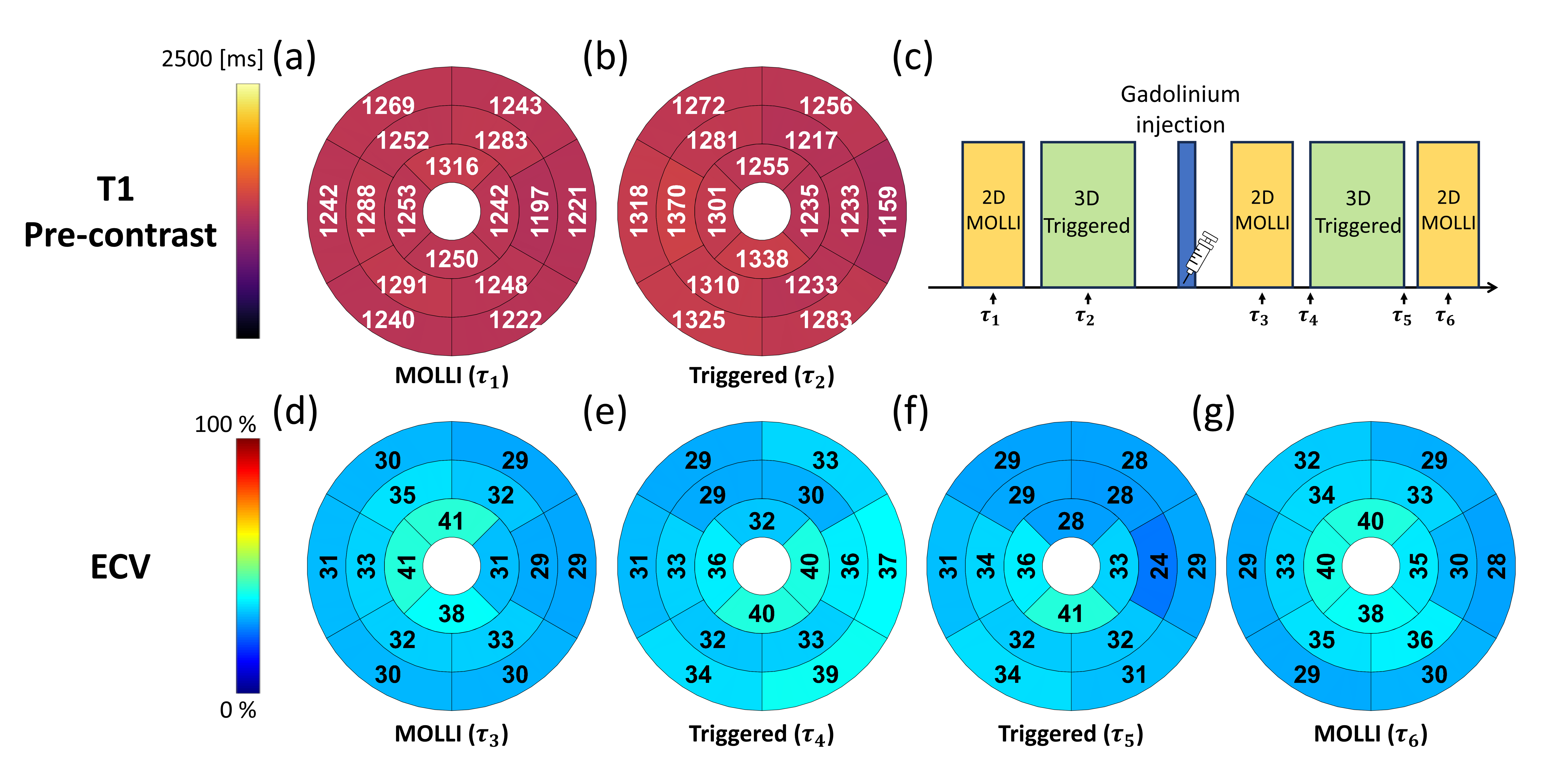
Figures 2 to 4 show the results of pre-contrast $$$T_1$$$, post-contrast $$$T_1$$$, and ECV maps, respectively. 3D pre-contrast $$$T_1$$$, post-contrast $$$T_1$$$, and ECV maps were successfully generated for the whole heart using the proposed method. Qualitatively, the estimated pre-contrast $$$T_1$$$, post-contrast $$$T_1$$$, and ECV were comparable to those acquired from MOLLI. Figure 5 shows the group results of Bull’s eye plots for pre-contrast T1 and ECV. Results show that the estimated pre-contrast $$$T_1$$$ and ECV were comparable to those acquired from MOLLI quantitatively (Fig. 5).

Conclusion

The proposed method allowed free-breathing, 3D ECV mapping in a practically feasible imaging time. The estimated ECV values from the proposed method were comparable to those from the existing method.

Acknowledgements

This work was supported in part by the National Institutes of Health (K01EB030045, P41EB022544, R01CA165221, R01EB033582, R01HL137230, and T32EB013180).