1445
Preliminary study of a receive Multi-Loop Coil (MLC) array for 7T brain MRI1Université Paris-Saclay, CEA, CNRS, Inserm, BioMaps, Orsay, France, Metropolitan, 2Université Paris-Saclay, CEA, Joliot, NeuroSpin, BAOBAB, Gif-sur-Yvette, France, Metropolitan, 3Multiwave Imaging SAS, Marseille, France, Metropolitan, 4Thales Research & Technology, Palaiseau, France, Metropolitan
Synopsis
Keywords: RF Arrays & Systems, RF Arrays & Systems
Motivation: The use of MLCs has shown the potential to improve the SNR at short distance as compared to an equivalent SLC.
Goal(s): Evaluation of the performances of a 8-channels MLC-array for head imaging at 7T.
Approach: Electromagnetic simulation was used to evaluate and compare the SNR, noise-covariance matrix and g-maps obtained with the MLC-array and with an equivalent array of SLC.
Results: As compared to the SLC-array, the MLC-array achieves an increased SNR in a relatively large peripheral ring and a reduced maximum g-factor.
Impact: Array of MLC represents a valuable strategy for array developpement at high field that can be employed to improve the SNR or reduce the number of channels.
Introduction:
Radio-frequency (RF) reception coils play a critical role in the MRI signal detection chain. Several studies have shown that employing dense arrays of small coils enhances signal-to-noise ratio (SNR) at the surface of the sample without SNR loss at the center1,2. Nevertheless, improvements associated with the coil size reduction are limited by the coil noise dominance3, and the high number of channels leads to increased cost and complexity. SNR can also be improved by the use of flexible coils, which fit closely the body surface and maximize signal detection4. In this work, we investigate a new RF coil array for 7T brain MRI whose elements are based on the Multi-Loop Coil (MLC) principle5 consisting in several loops operated in series. MLCs have shown the potential to improve the sensitivity at short distance compared to equivalent Single-Loop Coil (SLC). Their use in an array is expected to achieve high detection sensitivity in the peripheral brain region.Materials and Methods:
We focused on a single row of eight elements geometrically decoupled, curved and placed around a spherical phantom (σ = 0.7 S/m, εr = 75) with a diameter of 165 mm. In the context of simulating a prototype coil array, the elements were positioned close to the phantom, at distances of 1.5 mm or 1.8 mm as shown in Fig.1A-B.We propose a new design for MLC, which includes an overlap between the loops (Fig.1C) to eliminate signal-free regions. This MLC is made of four loops with an inner radius r of 13 mm and a conductor width of 1 mm. The distance d between the center of the MLC and the center of the loops is 26.5 mm. Performances of the MLC-array were compared in simulation to those of a classical array made of SLCs with a radius R of 47 mm, covering approximately the same surface as the MLCs (Fig.1D).
Performances of the investigated arrays were evaluated by 3D electromagnetic simulations using HFSS (ANSYS). All coils were tuned at 297.2 MHz using circuit co-simulation and matched to 50 Ω with a PI-matching network6. RF magnetic field B1- maps and S-parameters were extracted and post-processed using Matlab to calculate the noise correlation matrix, g-maps and SNR maps7.
Results:
Simulated SNR maps for SLC and MLC arrays are shown in Fig.2. The mean SNR in the central volume, outlined by the pink lines, shows a global improvement of the SNR by 4.8%. Fig.3A displays the SNR profiles along the dashed straight lines in Fig.2. The MLC-array achieves 10% higher SNR than the SLC-array in a large peripheral ring (40-mm width), but exhibits a 3% lower SNR in the central disk (20-mm radius). Fig.3B shows SNR-mean profiles along the azimuthal direction (dashed circular lines in Fig.2). The mean is computed across the solid segments in the peripheral ring where the MLC-array achieves higher SNR (17% average) than the SLC-array.The noise correlation matrix off-diagonal elements show mean/maximum values of 0.018/0.025 and 0.025/0.047 for the MLC and SLC arrays respectively. G-maps displayed in Fig.5 show similar values for the two arrays, but in most cases, maximum g-factors are significantly lower for the MLC-array.
Discussion and conclusion:
An 8-MLC receive array was simulated and compared to an equivalent SLC array. Its performance demonstrated a noticeable improved SNR in a peripheral ring inside the sample and a slight SNR decrease at the center. This is similar to the SNR increase observed when using an array with a higher number of channels and smaller elements, while in the present study, the MLC and SLC arrays have the same number of channels.This improvement is also visible on the g-maps. The MLC-array shows lower average and maximum g-factors as compared to the SLC-array. The MLC principle, due to the high sensitivity of the small loops, appears to be interesting to design arrays with increased peripheral SNR without the need to increase the number of channels.
The next step will be dedicated to MLC-array prototyping and validation at the MRI scanner. It would also be worthwhile to simulate an array with more elements and a realistic phantom head. Additional improvements could also be achieved with the development of other MLC geometries with different number of loops, placement, and various loop sizes.
Finally, coil arrays on flexible caps have been proposed with High-Impedance Coils (HIC)8,9. These are less sensitive to load variations as the head size varies. The use of HIC MLCs could enable to make use of the high sensitivity of MLCs without the limitation of performance dependence on the head size.
Acknowledgements
No acknowledgement found.References
1. Roemer, P. B., et al. The NMR phased array. Magn Reson Med 16, 192–225 (1990).
2. Gruber, B., et al. A 128-channel receive array for cortical brain imaging at 7 T. Magn Reson Med 90, 2592–2607 (2023).
3. Kumar, A., et al. Noise figure limits for circular loop MR coils. Magn Reson Med 61, 1201–1209 (2009).
4. McGee, K. P., et al. Characterization and evaluation of a flexible MRI receive coil array for radiation therapy MR treatment planning using highly decoupled RF circuits. Phys. Med. Biol. 63, 08NT02 (2018).
5. Frass-Kriegl, R., et al. Multi-Loop Radio Frequency Coil Elements for Magnetic Resonance Imaging: Theory, Simulation, and Experimental Investigation. Front. Phys. 7, (2020).
6. Wang, W., et al. Three-element matching networks for receive-only MRI coil decoupling. Mag Reson Med 85, 544–550 (2021).
7. Pruessmann, K. P., et al. SENSE: Sensitivity encoding for fast MRI. Mag Reson Med 42, 952–962 (1999).
8. Cogswell, P. M., et al. Application of Adaptive Image Receive Coil Technology for Whole-Brain Imaging. Am. J. Roentgenol. 216, 552–559 (2021).
9. Gapais, P-F., et al. A 32-Channel Cap for Temporal Lobes Exploration at 11.7 T, ISMRM 2024, Singapore.
Figures
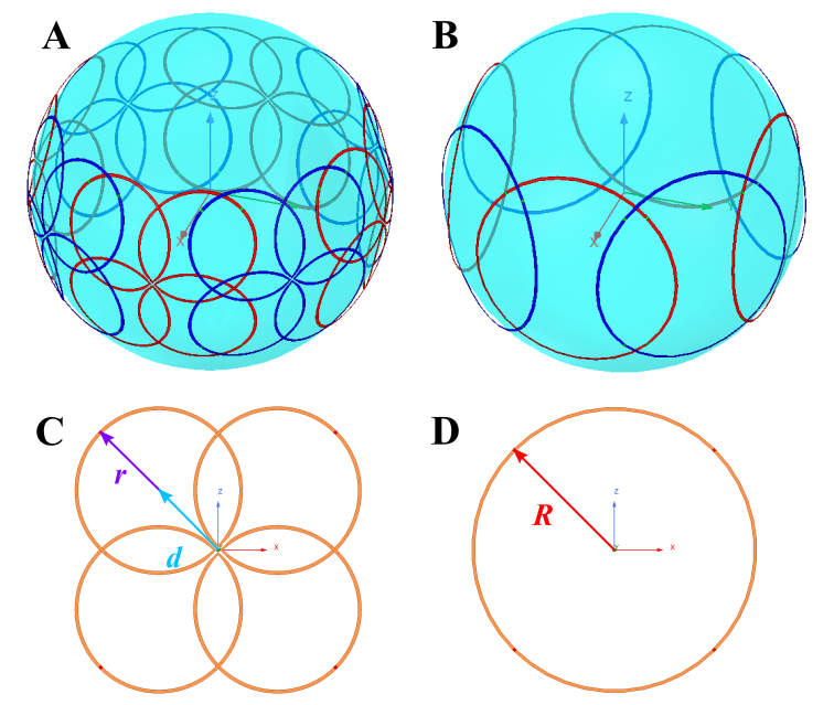
Figure 1 : Drawing of an 8 elements MLC-array (A) and SLC-array (B) with blue and red elements positioned at a distance of 1.8 mm and 1.5 mm from the phantom, respectively. Schematic of an MLC (C) and SLC (D) element, with 'R' being the radius of the SLC, 'd' the distance between the center of the MLC and the center of the loops, and 'r' the radius of the loops.
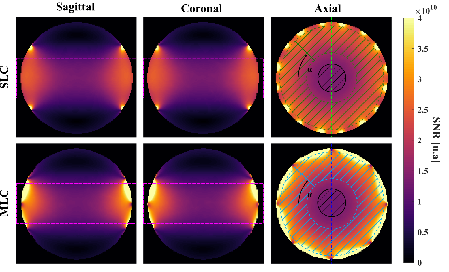
Figure 2 : Orthogonal views of the simulated SNR maps in a 165mm-diameter phantom (σ = 0.7 S/m, εr = 75) for the SLC and MLC arrays. The dotted lines and rings are used to draw the SNR curves displayed in Fig. 3. In the peripheral ring (light blue and dark green striped areas) the SNR increases by 17% in average with the MLC-array compared to the SLC-array. In the central black disk, the SNR decreases by 3% with the MLC compared to SLC-array. The mean SNR values were also computed in the central volume outlined by the dashed pink lines: there the MLC-array provides 4.8% more SNR than the SLC-array.
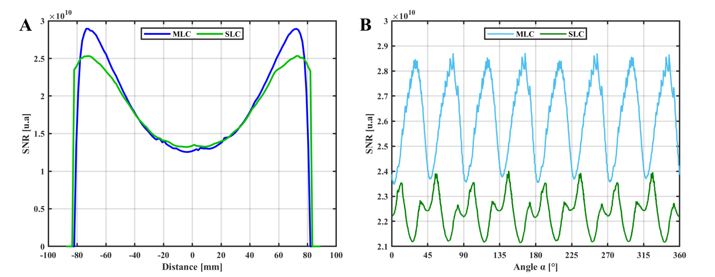
Figure 3 : SNR profiles along the dashed dark blue and light green lines in Fig.2 are shown in A: MLC’s SNR performs 10% better in average than SLC. In a large peripheral ring of 40mm-width, the MLCs achieve higher SNR. Inside this ring, the mean SNR across the solid dark green and light blue segments in Fig.2 are shown in B along the azimuthal direction. The MLC provides mean and max values respectively 17% and 32% better than the SLC.
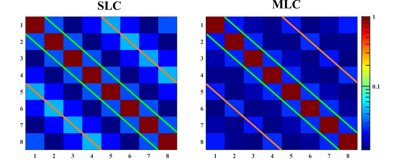
Figure 4 : Simulated noise correlation matrices from the MLC and SLC arrays displayed with a log scale. The adjacent coils (below the green lines) and the opposite coils (below the orange lines) are less correlated for the MLC array than for the SLC.
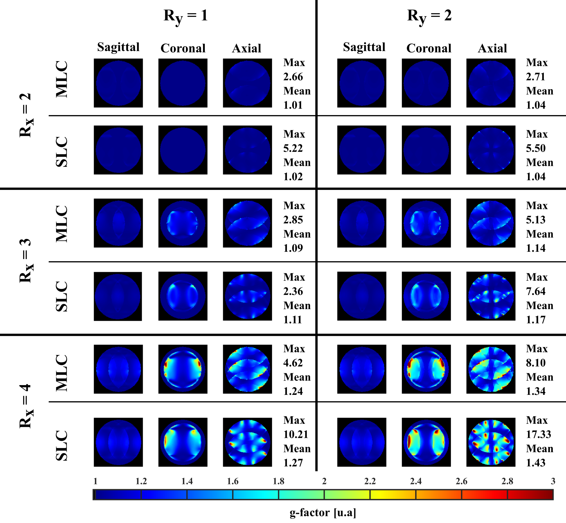
Figure 5 : Simulated g-maps in three orthogonal planes for various in-plane SENSE acceleration factor (Rx and Ry) for the two investigated arrays. In general, average and maximum g-maps are lower for MLC than for SLC array.