Introduction

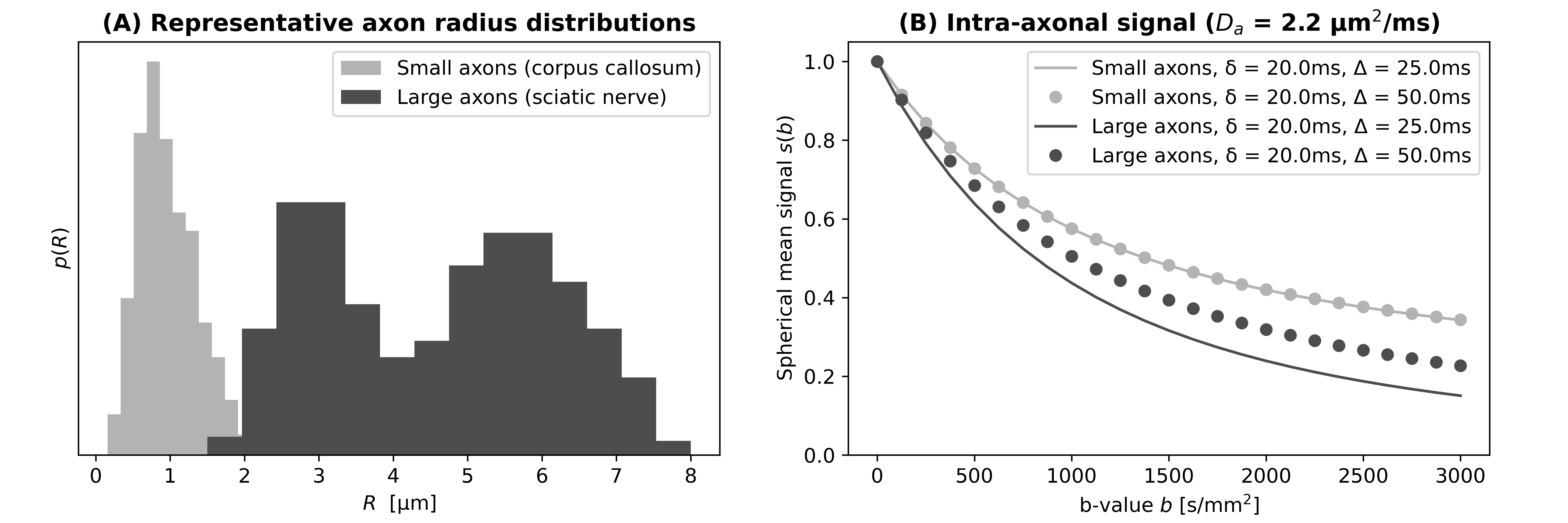
The stick (zero-radius cylinder) is a common diffusion-weighted (DW) signal model used for axons^1-5. The model is suitable for radii up to approximately 3 µm in clinical systems⁶, i.e., for most brain white matter. However, a mixture of small and large axons is found in the peripheral nervous system (PNS⁷; radii as large as 8 µm). For such large axons, the DW signal deviates from the idealised stick signal⁸, featuring stronger attenuation and diffusion-time dependence (Fig. 1). This may bias the estimation of key microstructural parameters such as the intra-axonal (IA) signal fraction $$$f_a$$$, a promising marker of axonal loss. To address this issue, we investigated the feasibility of replacing the stick model with a two-axon population (TAP) approach accounting for large axons. Specifically, we compared TAP and stick signal modelling in simulations, and tested the application of TAP in the PNS in vivo.

Methods

Simulations
We compared $$$f_a$$$ estimates of IA signal fraction obtained through both TAP and standard “stick” modelling in synthetic signals.

Signal synthesis We synthesised the total DW signal by summing IA and extra-axonal (EA) signal contributions ($$$s_a$$$ and $$$s_e$$$) as


$$s\,\,=\,\,f_a \,s_a\,\,+\,\,(1-f_a)\, s_e.\,\,\,\,\,(1)$$

$$$s_a$$$ integrates contributions from a distribution of axonal radii, i.e.,

$$s_a\,\,=\,\, c\int_{0}^{\infty}R^2\,h(R,D_a,b,\delta,\Delta)\,p(R;\eta,\zeta)\,dR.\,\,\,\,\,(2)$$

Above, $$$p(R;\eta,\zeta)$$$ is a gamma distribution^8,9 (shape: $$$\eta$$$; scale: $$$\zeta$$$; mean: $$$R_m=\eta\,\zeta$$$; variance: $$$R_{s}^{2}=\eta\,\zeta^2$$$), and $$$c$$$ ensures $$$s_a(b=0)=1$$$. $$$h(R,D_a,b,\delta,\Delta)$$$ is the powder-averaged signal^4,10 for diffusion within a cylindrical axon of radius $$$R$$$ and IA diffusivity $$$D_a$$$, i.e.,

$$h(R,D_a,b,\delta,\Delta)\,\,=\,\frac{\sqrt{\pi}}{2}\,e^{-b\,D_p(R,D_a,\delta,\Delta)}\,\frac{\mathrm{erf}\Big( \sqrt{b\big(D_a - D_p(R,D_a,\delta,\Delta)\big)} \Big)}{\sqrt{b\big(D_a - D_p(R,D_a,\delta,\Delta)\big)}}.\,\,\,\,\,(3)$$

Above,

$$D_p(R,D_a,\delta,\Delta)\,\,=\,\,\frac{2}{D_a\delta^2(\Delta-\delta/3)}\,\sum_{m=1}^{\infty}\,\frac{\big(2D_a\alpha_m^2\delta\,-2\,+2e^{-D_a\alpha_m^2\delta}\,+2e^{-D_a\alpha_m^2\Delta}\,-e^{-D_a\alpha_m^2(\Delta-\delta)}\,-e^{-D_a\alpha_m^2(\Delta+\delta)}\big)}{\alpha_m^6(R^2\alpha_m^2-1)}\,\,\,\,\,(4)$$

is the IA perpendicular apparent diffusion coefficient (ADC)¹¹, and $$$\alpha_m$$$ indicates the roots of $$$J_{1}^{'}(\alpha_m R) = 0$$$. Finally, the EA signal is generated as

$$s_e\,\,=\,\,e^{-b\,D_e},\,\,\,\,\,(5)$$

where $$$D_e$$$ is the EA ADC.

We synthesised signals for 1500 uniformly-distributed combinations of $$$f_a$$$, $$$D_a$$$, $$$D_e$$$, $$$R_m$$$, $$$R_s$$$ ([0; 1], [1.0; 3.0] µm²/ms, [0.5; 3.0] µm²/ms, [1; 6] µm, [0.3$$$R_m$$$; 0.7$$$R_m$$$]). The protocol was b = {0, 500, 1000, 1500, 2000, 2500, 3000} s/mm² × Δ = {30, 50, 70} ms (fixing δ = 20ms). Signals were corrupted with Rician noise (b=0 signal-to-noise-ratio: 20).

$$$f_a$$$ estimation We fitted an IA/EA model

$$ s\,\,=\,\,f_a\,s_a\,\,+\,\,(1-f_a)\,e^{-b\,D_e},\,\,\,\,\,(6)$$

comparing two implementations of $$$s_a$$$:

- TAP: $$$s_a$$$ is written as

$$s_a\,\,=\,\,f_l\,h(R_l,D_a,b,\delta,\Delta)\,\,+\,\,(1-f_l)\,h(0,D_a,b,\delta,\Delta),\,\,\,\,\,(7)$$

to include a mixture of "sticks" and large axons, with signal fraction $$$f_l$$$ and characteristic radius $$$R_l$$$. Note that in the “stick” model $$$h(0,D_a,b,\delta,\Delta)$$$ the IA perpendicular ADC vanishes, since in Eq. 4 above, $$$D_p(R,D_a,\delta,\Delta) \rightarrow 0$$$ for $$$R \rightarrow 0$$$.

- Stick: $$$s_a$$$ follows the standard zero-radius model

$$s_a\,\,=\,\,h(0,D_a,b,\delta,\Delta).\,\,\,\,\,(8)$$

Estimated/reference $$$f_a$$$ were compared through bias and dispersion (variability) indices.

In vivo demonstration
We investigated TAP modelling in vivo by analysing retrospectively sciatic nerve scans from 24 healthy volunteers (mean age 36.4 years, range 26-53, 17 female) and 23 people with relapsing-remitting multiple sclerosis (RRMS; mean age 40.0 years, range 30-59, 13 female). DW images, acquired at 3T (Philips Ingenia CX, b = {0, 700, 1200, 2000} s/mm², δ = 15.06 ms, Δ = 37.55 ms, resolution 1×1×10 mm³, TE=80 ms; TR=4000 ms), were pre-processed^12,13, and $$$D_e$$$, $$$f_a$$$ and $$$f_l$$$ computed. Mean values within the manually-segmented sciatic nerve were compared between groups via linear regression, adjusting for age, gender, and body mass index.

Results and discussion

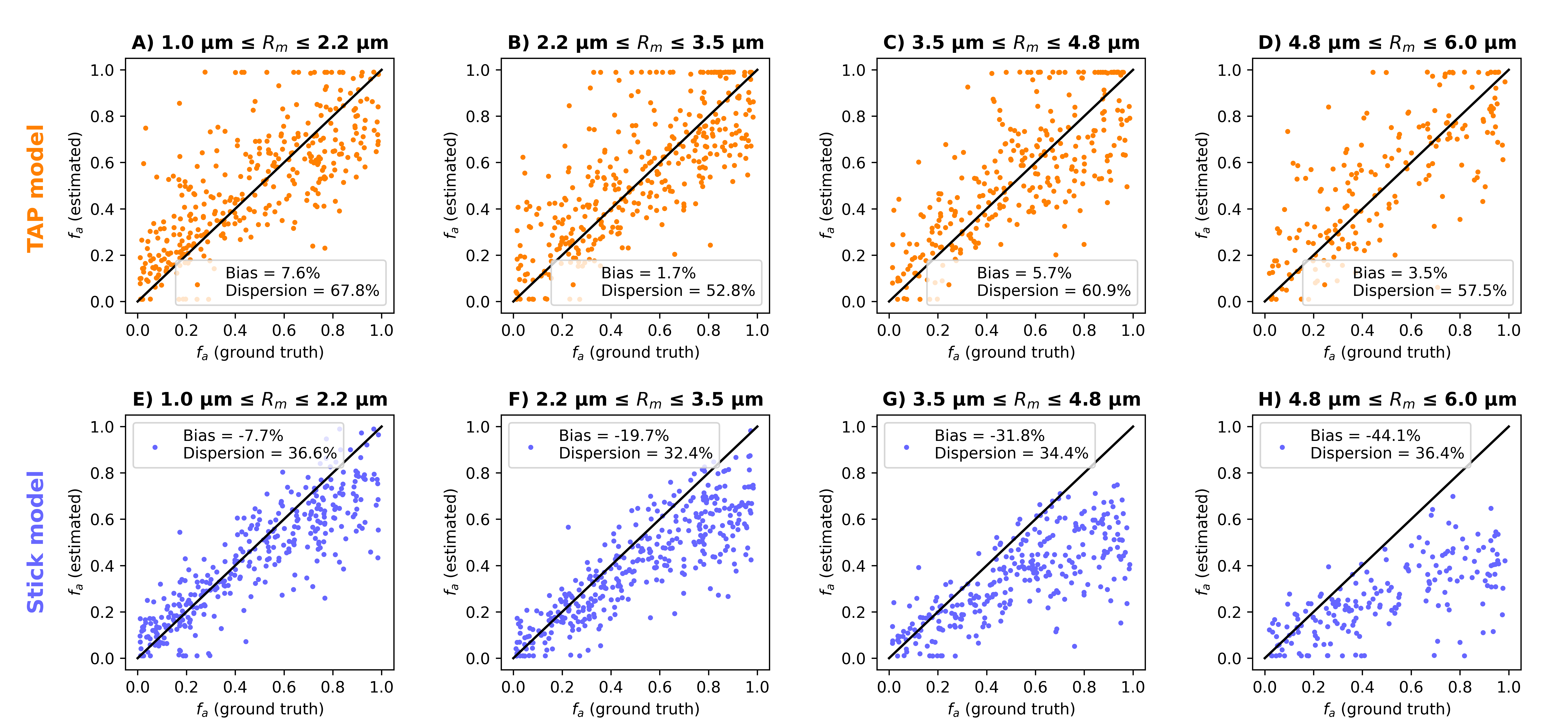
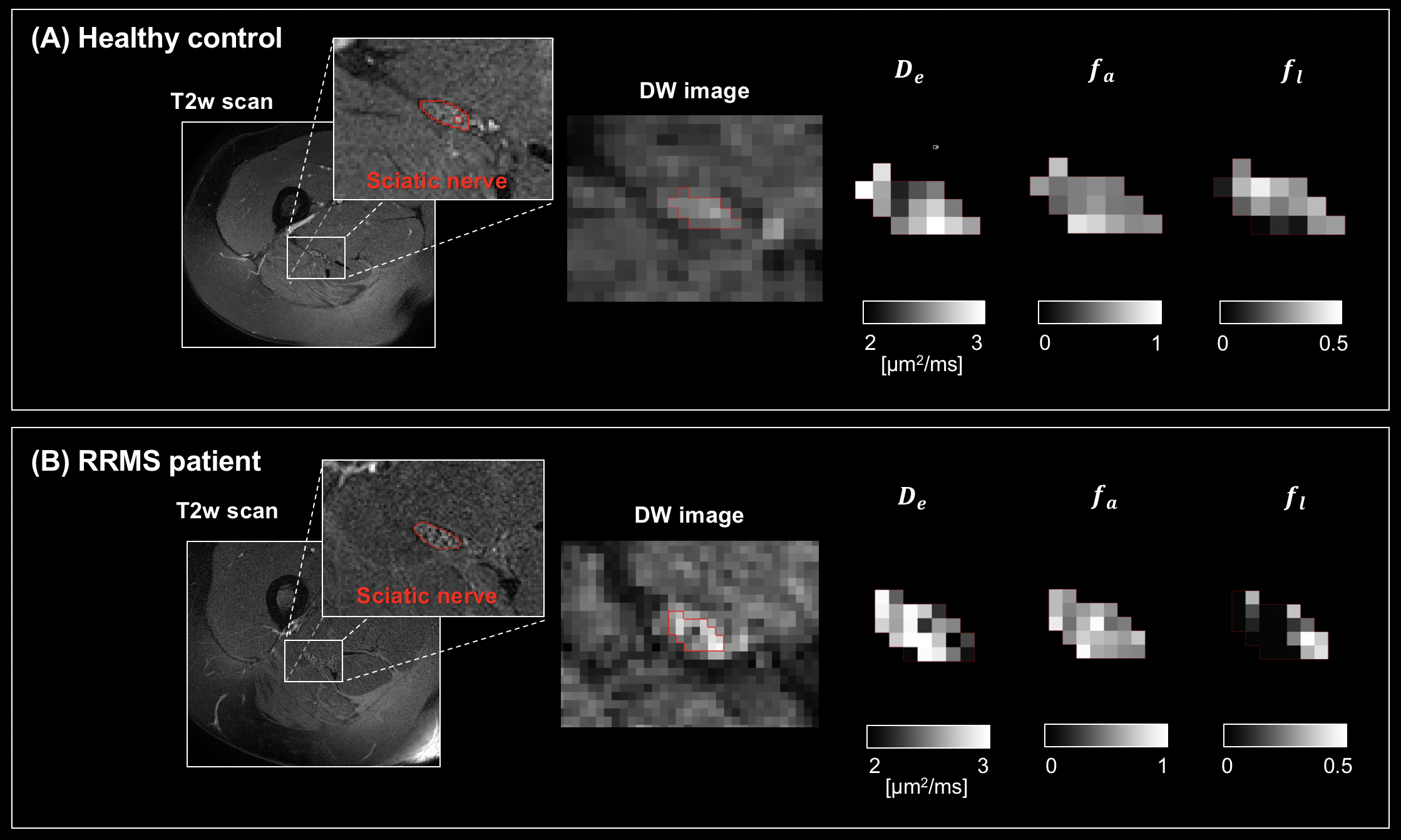
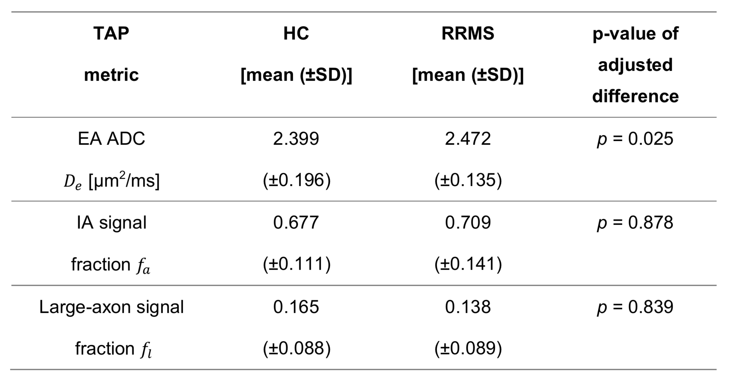
Fig. 2 shows scatter plots visualising $$$f_a$$$ predictions for axons with increasingly large mean radius $$$R_m$$$. For the smallest axons, both TAP and the stick models provide accurate estimates of $$$f_a$$$. However, as $$$R_m$$$ increases, stick estimates become increasingly biased, underestimating ground truth $$$f_a$$$, unlike TAP. This result points towards the need for accounting for finite axon radius in the presence of large axons. Finally, TAP $$$f_a$$$ shows higher variability than stick estimates, owing to the increased number of unknown tissue parameters, which makes TAP more difficult to fit than the stick model.

Fig. 3 shows examples of TAP maps $$$D_e$$$, $$$f_a$$$ and $$$f_l$$$ in vivo in a representative control and a representative RRMS patient, while Table 1 reports mean/standard deviation values in the two groups. In both patients and controls, voxels with high $$$f_l$$$ values, consistent with the presence of a significant number of large axons, are seen. Statistically significant patient-control differences are observed for the EA ADC $$$D_e$$$, with higher $$$D_e$$$ in patients than in controls (p = 0.025), compatible with early demyelination. This finding suggests that TAP metrics may be useful biomarkers for non-invasive neurophysiological assessment of PNS microstructure, as in MS applications.

Conclusions

TAP modelling can reduce biases in IA signal fraction estimation in the presence of large axons. It provides microstructural metrics that may become useful biomarkers in PNS applications, as in the characterisation of preferential large/small axon degeneration.

Acknowledgements

FG and RB are joint first authors with equal contribution. This work is financially supported by the National Brain Appeal’s Innovation fund (https://www.nationalbrainappeal.org). FG receives the support of a fellowship from ”la Caixa” Foundation (ID 100010434). The fellowship code is “LCF/BQ/PR22/11920010”. RB receives a scholarship from Chiang Mai University, Chiang Mai, Thailand. CGWK receives funding from Horizon 2020 (Research and Innovation Action Grants Human Brain Project 945539 (SGA3)), BRC (#BRC704/CAP/CGW), MRC (#MR/S026088/1), Ataxia UK, Rosetrees Trust (#PGL22/100041 and #PGL21/10079). CGWK is a shareholder in Queen Square Analytics Ltd.