Introduction

Proton resonance frequency shift (PRFS) thermometry is the current standard for MR-based temperature monitoring in interventional procedures. It measures phase changes due to frequency changes with temperature [1]. However, the relatively long TE required for the PRFS method leads to signal dropout in heated regions as T₂ shortens and T₁ lengthens with heating. Additionally, PRFS acquisitions can have poor SNR efficiency and high sensitivity to physiological and other spurious motion. Quadratic RF phase MR fingerprinting (qRF-MRF) can also quantify off-resonance using much shorter TEs and has a very high SNR efficiency, and thus has the potential to generate high-precision temperature maps [2]–[4]. Here we report a dynamic qRF-MRF pulse sequence and model-based image and continuous sliding window temperature map reconstruction for high temporal resolution and demonstrate its precision in vivo and its ability to monitor focused ultrasound heating.

Methods

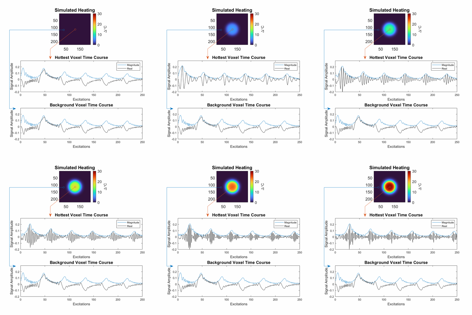
Pulse Sequence Mechanism

The qRF-MRF thermometry sequence works by continuously sweeping the RF excitation phase of a constant low-flip-angle as illustrated in Figure 1. The resonance frequency continuously sweeps from -1/TR to +1/TR Hertz in a short-TE/short-TR bSSFP sequence. Fig 1 shows that voxels with different temperatures or off-resonance frequencies will then generate distinct signal time courses, which can be matched to a Bloch-simulated dictionary to quantify off-resonance. We used Monte Carlo simulations with random noise added to optimize the sequence parameters, including the ramp of the quadratic RF phase and flip angle.

Scanner Implementation

The qRF-MRF thermometry sequence was implemented on a 3T (Vida, Siemens Healthcare) scanner, using a 16-channel Rx coil and a spiral-out readout. A constant TR = 10 ms, TE = 2.5 ms, and flip angle = 10° were used with a quadratically increasing 4.2n² RF phase to continuously cycle the sequence’s resonance frequency from -50 to +50 Hz range. Conventional 2DFT PRF temperature maps were also acquired using a 12 ms TE gradient echo sequence, generating a dynamic image every 2.2 seconds. Both sequences had 256x256 mm² FOVs and 2 x 2 x 5 mm³ resolution.

Temperature Reconstruction
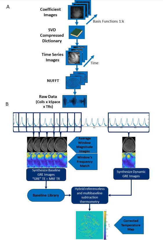
A dictionary was constructed for a single brain tissue-like T₁/T₂ pair (825 ms, 70 ms), a range of off-resonances (-50 Hz to 50 Hz), and 21 Gaussian linewidths (1 to 51 Hz). Temperature maps were reconstructed dynamically over 1-3 second-long sliding time windows. Images within each window were jointly reconstructed using a dictionary-constrained algorithm that solved for coefficient maps in an SVD-compressed-dictionary subspace; the forward model is illustrated in Figure 2A. A temperature map was generated from a window’s frequency map by synthesizing a GRE image with TE equal to the qRF-MRF TR to match phase wraps, and then applying the hybrid referenceless multibaseline subtraction thermometry method Figure 2B [5].

Experiments

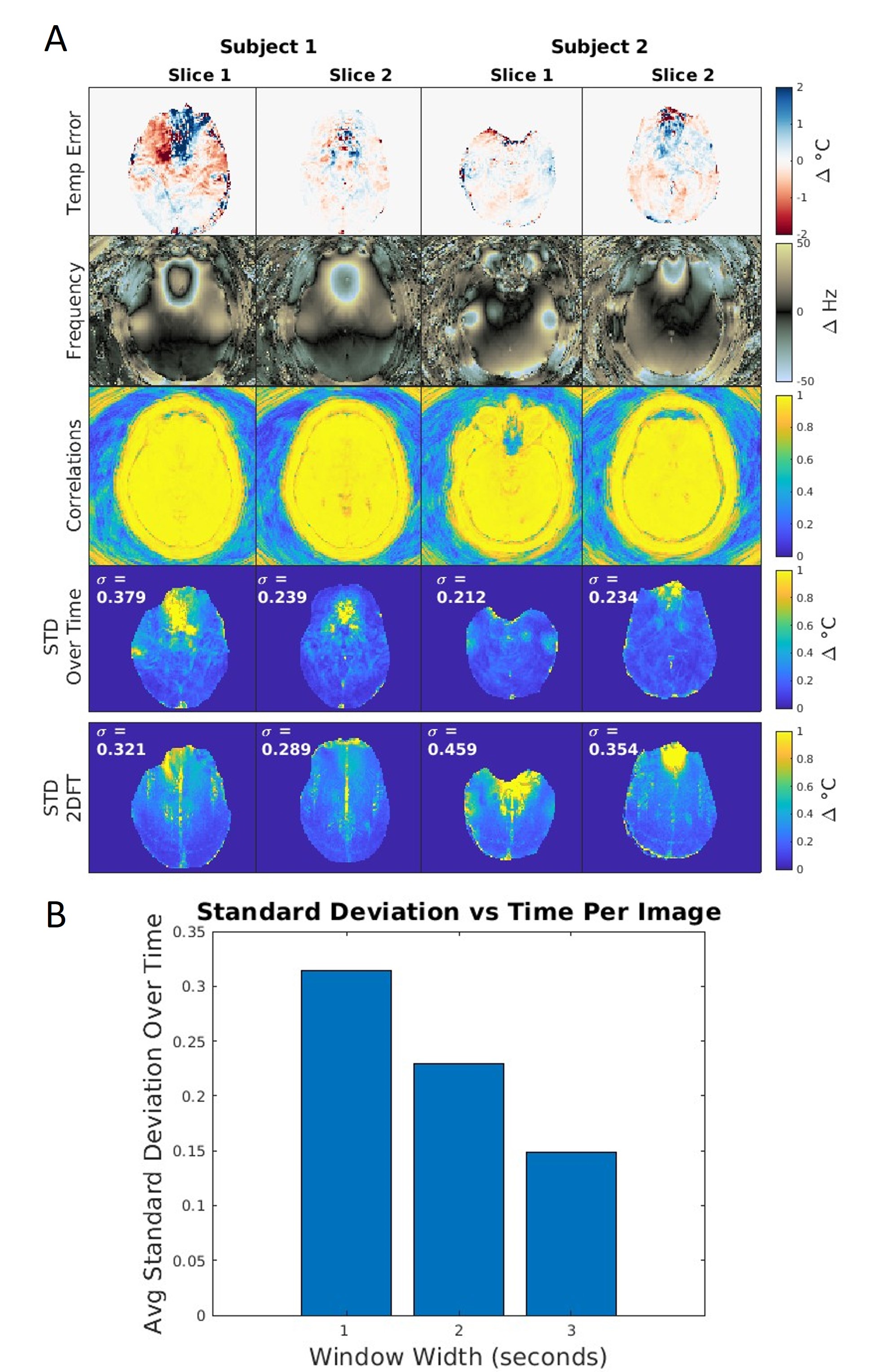
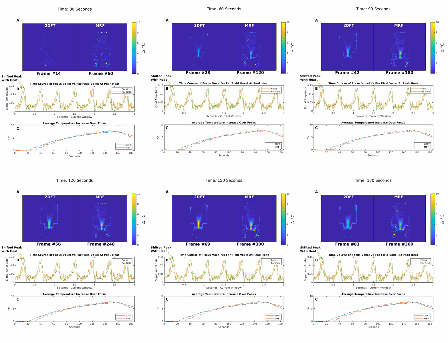
In vivo healthy subject scans without heating were conducted in accordance with local IRB, acquiring two slices covering the hippocampus and thalamus in two subjects, measured over several minutes to enable comparison of 2DFT and qRF-MRF temperature precision (Figure 3). In a phantom, a heating experiment was performed using a focused ultrasound transducer (H115MR, Sonic Concepts) at 250 mV pp for 2 minutes. The phantom was a 1% agar weight by volume of water for the coupling medium and a 1% agar / 4 % graphite weight by volume for the main body of the phantom. The qRF-MRF data were reconstructed with 300 TRs per dynamic time point, updated every 0.5 seconds (Figure 4)

Results and Discussion

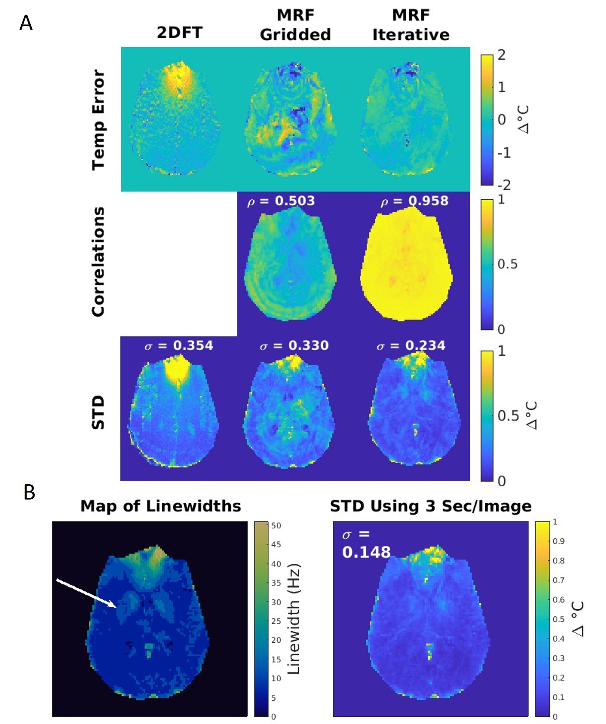
Figure 3 shows data for 2 different slices in 2 subjects and a comparison of precision between 2DFT and MRF, measured as standard deviation over time; the qRF-MRF has improved temperature precision in nearly every case, for the same scan time. Figure 4 compares temperature maps of the heated phantom, both showing similar values for peak heating. The qRF-MRF method provides temperature maps with much higher (>4x here) temporal resolution due to the sliding window reconstruction. Figure 5A shows a comparison of temperature error and dictionary match correlations between the 2DFT, gridded qRF-MRF, and iterative recon qRF-MRF; the iterative recon yields improved temperature precision and greater certainty in frequency matching. Figure 5B shows maps of Gaussian linewidths and through-time standard deviations from a qRF-MRF reconstruction; areas with wider linewidths correspond to areas with higher temperature uncertainty. Also shown clearly in the linewidth map are high-iron regions such as the putamen.

Conclusion

qRF-MRF temperature mapping enables high spatiotemporal resolution thermometry with improved precision compared to 2DFT acquisitions. Future work will focus on evaluating relative sensitivity to spurious artifacts such as from water bath motion in FUS ablation.

Acknowledgements

This work was supported by NIH grants R01 NS120518 and R01 EB028773.

References

[1] V. Rieke and K. Butts Pauly, “MR thermometry,” J. Magn. Reson. Imaging, vol. 27, no. 2, pp. 376–390, Feb. 2008, doi: 10.1002/jmri.21265. [2] R. Boyacioglu, M. Poorman, K. Keenan, and M. Griswold, “Magnetic Resonance Fingerprinting with Quadratic RF Phase for Continuous Temperature Monitoring in Aqueous Tissues,” Proc. Intl. Soc. Mag. Reson. Med. 28 (2020). [3] K. Keenan, M. A. Griswold, M. E. Poorman, and R. Boyacioglu, “Magnetic Resonance Fingerprinting Thermometry,” US Patent No. 11519987 B2 [4] C. Y. Wang, S. Coppo, B. B. Mehta, N. Seiberlich, X. Yu, and M. A. Griswold, “Magnetic resonance fingerprinting with quadratic RF phase for measurement of T2* simultaneously with δf, T1, and T2,” Magnetic Resonance in Medicine, vol. 81, no. 3, pp. 1849–1862, 2019, doi: 10.1002/mrm.27543. [5] W. A. Grissom et al., “Hybrid referenceless and multibaseline subtraction MR thermometry for monitoring thermal therapies in moving organs: Hybrid MR thermometry in moving organs,” Med. Phys., vol. 37, no. 9, pp. 5014–5026, Aug. 2010, doi: 10.1118/1.3475943.