Introduction

Recent developments in bone MR imaging techniques include the generation of synthetic CT (sCT) contrast using deep learning models^1,2. However, generative models typically suffer from limited image sharpness, hindering the clinical applicability of sCT for diagnostic purposes. The blurriness of synthetic contrasts can be partly explained by the high energy contained in the low frequencies of the Fourier spectrum of images. This biases the standard intensity-based losses (e.g., L1, L2) and results in a poor estimation of higher frequencies. To overcome this limitation, the use of a focal frequency loss (FFL) has been recently proposed for computer vision applications by Jiang et al.³, and resulted in a more accurate depiction of high frequency details.

In this work, we investigate the use of FFL for the generation of sCT images from T1-weighted MRI and compare the results with a baseline model using L1 loss only.

Methods

Demographics, imaging protocols and pre-processing
A cohort of 418 subjects (from the Lausanne Knee Study, 47.2±16.2 years old, 231 females) was recruited and underwent both a 3T MRI (MAGNETOM Prismafit, Siemens Healthineers AG, Erlangen, Germany) including a T1-weighted 3D gradient-echo sequence (0.5mm isotropic, TR=700ms, TE=11ms), and a CT scan (0.3mm isotropic, Revolution, GE Healthcare).
The training of supervised generative models required an accurate correspondence between T1-weighted MRI and CT image pairs for each subject. To this end, the T1-weighted MRI images were spatially registered to down-sampled CT volumes applying a combination of rigid, affine and non-linear transformations with elastix⁴. Two independent readers evaluated the registration quality and only image pairs with the highest score were retained.

Synthetic CT generation
Training and test sets were obtained from the dataset, by selecting 90% and 10% of all image pairs, respectively.
As proposed by Jiang et al.³, the computation of the FFL relies on the L2 difference between Fourier spectra obtained from the sCT and the ground truth (noted $$$FT_{sCT}$$$ and $$$FT_{CT}$$$ hereafter). Additionally, a dynamic weighting scheme is applied to the voxel-wise differences in frequency domain, to assign higher weights to the regions in the Fourier spectra that display the greatest deviations from the ground truth. Therefore, the focal frequency loss can be expressed as:
$$
FFL = \sum_{\forall k}w[k] * ||FT_{sCT}[k] - FT_{CT}[k]||_2 ,
$$
with
$$
w[k] = |FT_{sCT}[k] - FT_{CT}[k] |
$$
denoting the weight associated with frequency $$$k$$$. The total loss of the proposed model can be summarized as:
$$
L=L1 + λ_{FFL}*FFL,
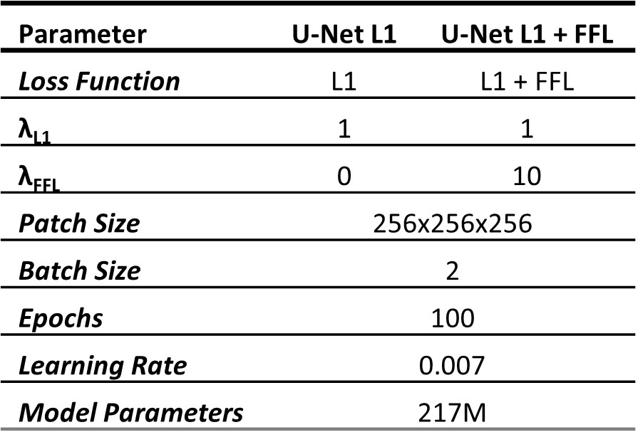
$$ with $$$L1(sCT, CT)=\sum_{\forall r}|sCT[r] - CT[r]|$$$, where $$$X[r]$$$ is the image intensity of image $$$X$$$ in voxel $$$r$$$. The results were compared with a baseline model trained to solely minimize the L1 loss. Table 1 reports the detailed training parameters.

Evaluation
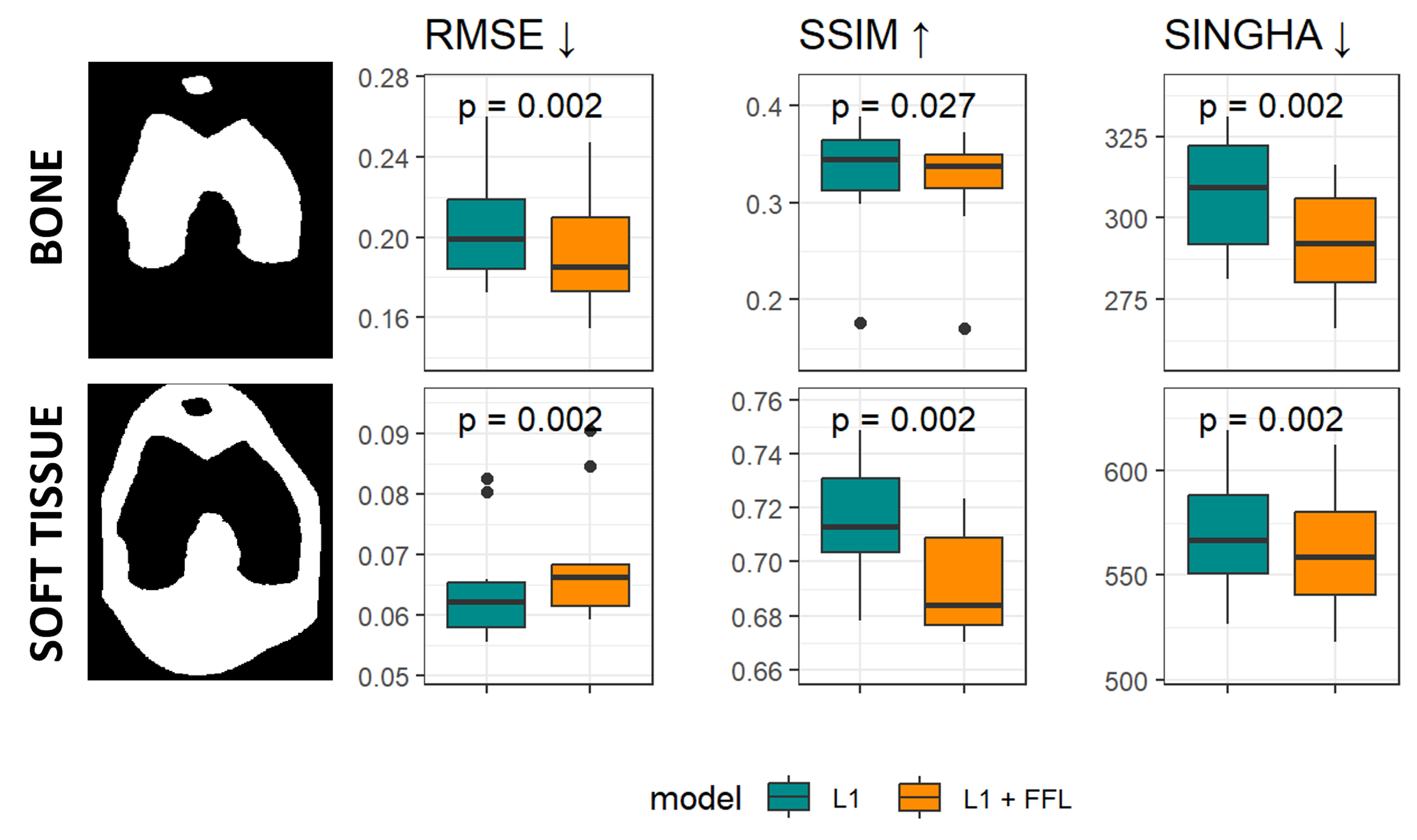
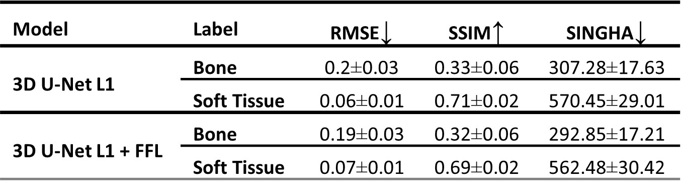
The accuracy of the sCT images was estimated on the test set inside the bone and in soft tissue. For a quantitative evaluation, standard intensity-based distortion metrics were assessed (i.e., structural similarity, SSIM and root mean squared error, RMSE), as well as a novel frequency-based metric dubbed SINGHA (Spectrally-INformed Grading of High-frequency Attributes)⁵. The latter was used to compare the high spatial frequency contributions between images, and was computed as a weighted sum over the magnitude spectrum that was averaged across frequencies at a common distance to the k-space centre, with higher weight for higher frequencies.
Accuracy metrics computed for both models were compared statistically using the Wilcoxon test for paired samples.

Results

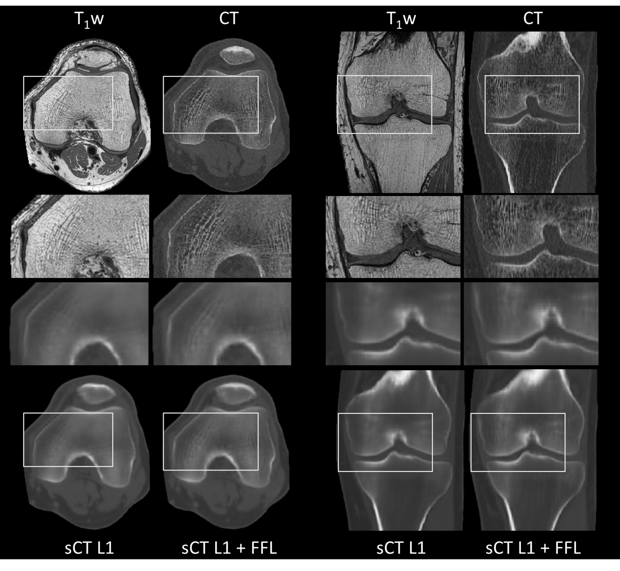
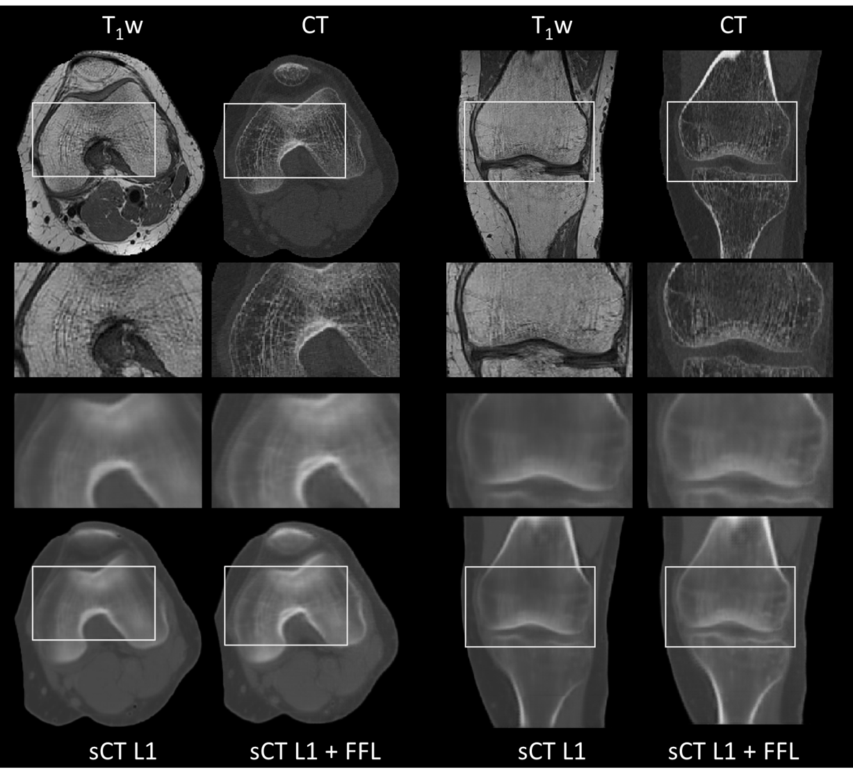
After visual inspection of the registration quality, 101 paired datasets were selected for training and test datasets. Figure 1 and Figure 2 show the sCT images obtained using both models in two example subjects. Qualitatively, the model using the FFL resulted in a higher level of details with increased image sharpness compared to the baseline model. Particularly, trabecular bone structures became more apparent, and the bone fascia was better delineated.

Figure 3 and Table 2 show the distribution of accuracy metrics for the two models across the test set. The use of the FFL led to very minor but statistically significant differences in RMSE compared to the baseline model and performed worse in terms of SSIM. However, lower SINGHA values were observed inside the bone for the FFL model, consistent with the visually perceived improvement in image sharpness.

Discussion and Conclusion

Our results suggest that using a frequency-based optimization function, such as a focal frequency loss, contributes to the improvement of image sharpness in image-to-image translation techniques. Therefore, a combination of intensity- and frequency- based loss functions could benefit the accuracy of synthetic contrast generation. Future work will investigate these findings in terms of clinical relevance of sCT for the characterization of bone pathology.

Acknowledgements

Lausanne Knee Study: Ethics approved and subjects gave their consent. This work was performed with the support of the Swiss National Science Foundation, Switzerland (Sinergia grant CRSII5_177155)