1189
Using Real Time Phase contrast MRI to investigate CSF oscillations and aqueductal pressure gradients during free breathing1Amiens Picardy University Hospital, CHIMERE UR.7516, Amiens, France, 2Jules Verne University of Picardy, CHIMERE UR 7516, Amiens, France, 3Amiens Picardy University Hospital, Neurosurgery Department, Amiens, France, 4Amiens Picardy University Hospital, Radiology Department, Amiens, France
Synopsis
Keywords: Head & Neck/ENT, Brain, aquduct, respiratory effects, real time imaging, phase contrast, intracranial pressure
Motivation: CSF dynamics is complex and regulates intracranial pressure. Pressure difference dynamics between the third and fourth ventricles (ΔPt) drives CSF oscillations in the aqueduct. MRI can quantify aqueduct anatomy and CSF oscillations.
Goal(s): To quantify ΔPt during free-breathing by combining MRI anatomical imaging with real-time phase-contrast MRI.
Approach: We developed a dedicated software to obtain: CSF flows dynamics Q(t), morphology of the aqueduct, its flow resistance (R) and ΔPt which equal R·Qt. Cardiac and breathing contributions to ΔPt were investigated in volunteers.
Results: Contributions to ΔPt were 12.3 Pa and 9.5 Pa from cardiac and breathing respectively.
Impact: Dedicated post-processing of real-time phase-contrast MRI allows quantification of CSF oscillations in the aqueduct and the pressure gradient between the third and fourth ventricles. Furthermore, continuous flow acquisition allows calculation of the cardiac and breathing influence on the pressure gradient.
Introduction
Cerebrospinal fluid (CSF) flow in the cerebral aqueduct is driven by the pressure difference (ΔP) between the third and fourth ventricles1. This ΔP can be calculated non-invasively by measuring the morphology of the aqueduct and the CSF flow through it2-4. However, precise morphological segmentation and post-processing of the images is currently a challenge for quantifying the ΔP. Furthermore, studies quantifying ΔP under breathing influence are lacking.For this purpose, we have developed a highly automated platform (IDL language) that allows accurate quantitative analysis of cerebral aqueductal morphologies. This study aimed to use this platform, combined with continuous flow curves obtained from real-time phase-contrast MRI (RT-PC)5,6, to quantify ΔP under cardiac and breathing influence.
Methods
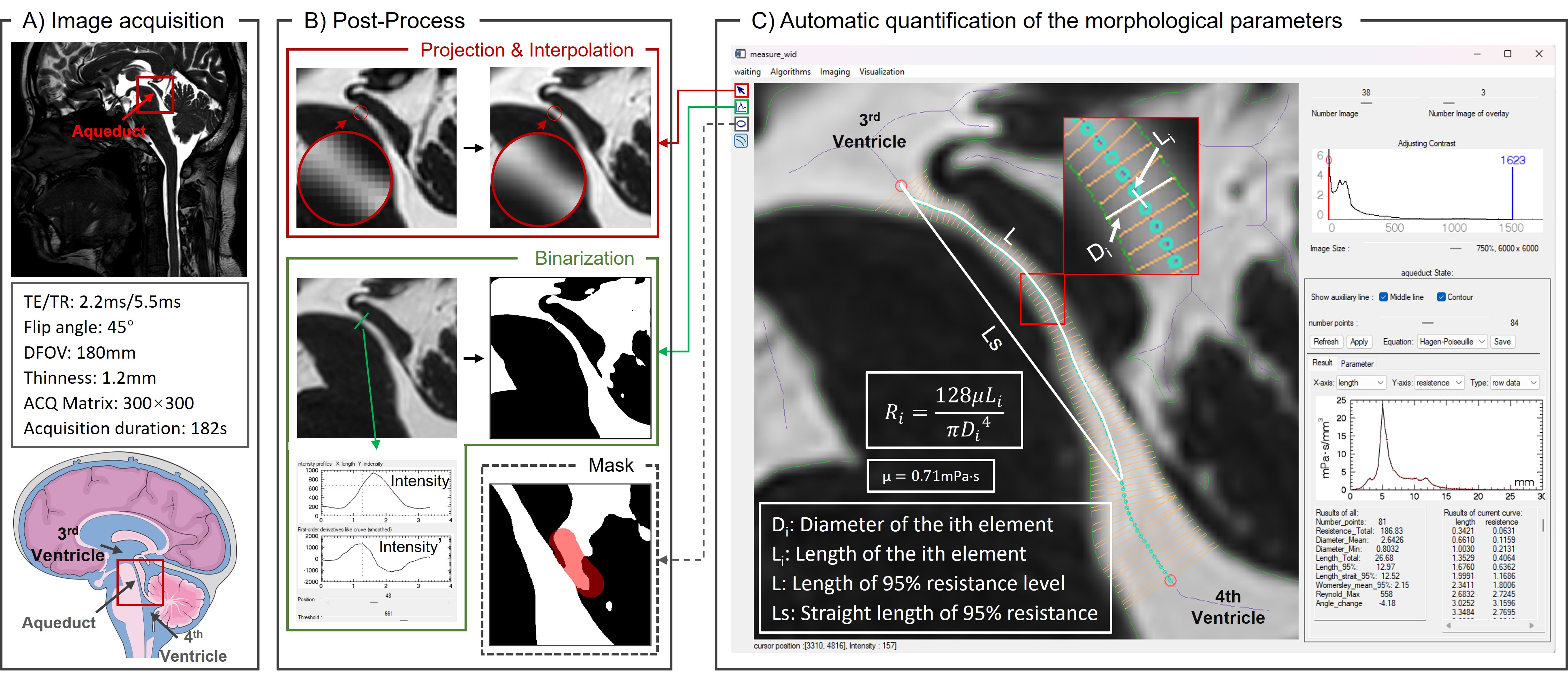
Thirty-four healthy volunteers (age: 19-35) were examined using a clinical 3T scanner and a 32-channel head coil.The cross-section of the aqueduct is nearly circular7, and the hydrostatic effects are still dominant. In this study, we employed a two-dimensional projection of the aqueduct for morphological analysis and applied the Poiseuille formula to calculate ΔP. The equation ΔP=R*Q comprises two crucial components: the resistance R (Fig.1-C) and the flow rate Q.
- Calculation of Resistance
The sagittal plane was imaged using the Balanced Fast Field Echo (BFFE) sequence with the parameters shown in Fig.1-A.
- 2-3 images were selected for merging to obtain the aqueduct projection, and then linear interpolation was applied to increase the spatial resolution to 0.03×0.03mm2.
- A line is manually drawn at the narrowest point of the aqueduct, and the software then automatically performs binary segmentation of the image based on the first-order derivative of the pixel's intensity profile.
- Optionally, the platform supports mask inclusions (Fig.1-B).
- The platform automatically delineates the boundary and centreline of the aqueduct, dividing it into multiple elements. Parameters such as length, diameter, angle, etc., are calculated for each element, along with its corresponding value of R (Fig.1-C).
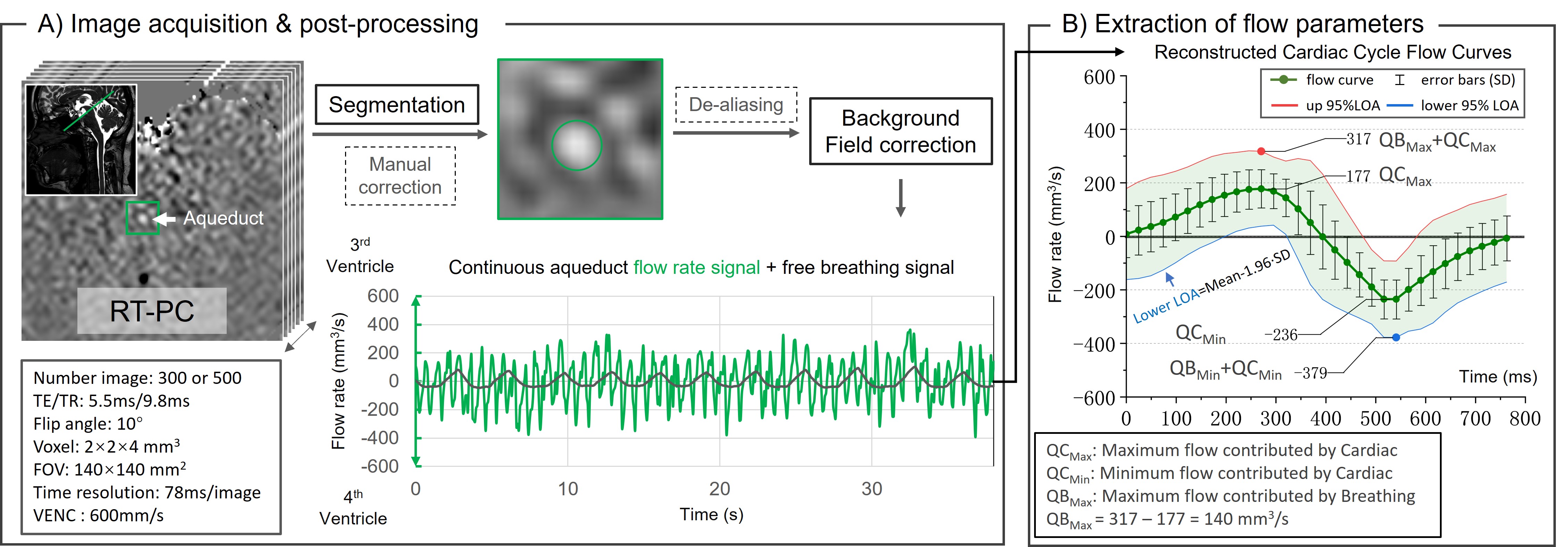
Using in-house Flow8-10 software for RT-PC post-processing:
- The continuous flow signal was extracted through post-processing steps including image segmentation, background field correction and de-aliasing.
- The flow signal was segmented into independent cardiac cycle flow curves (CCFC), interpolated to 32 points, and reconstructed into an average CCFC. The 95% limit of agreement (LOA) was calculated for this averaged CCFC (Fig.2-A).
- Cardiac-induced flow variations corresponded to the extremes of the CCFC (QCMin and QCMax). In contrast, Breathing-induced flow variations (QBMin and QBMax) were defined by the difference between the extremes of the LOA and the extremes of the CCFC (Fig.2-B).
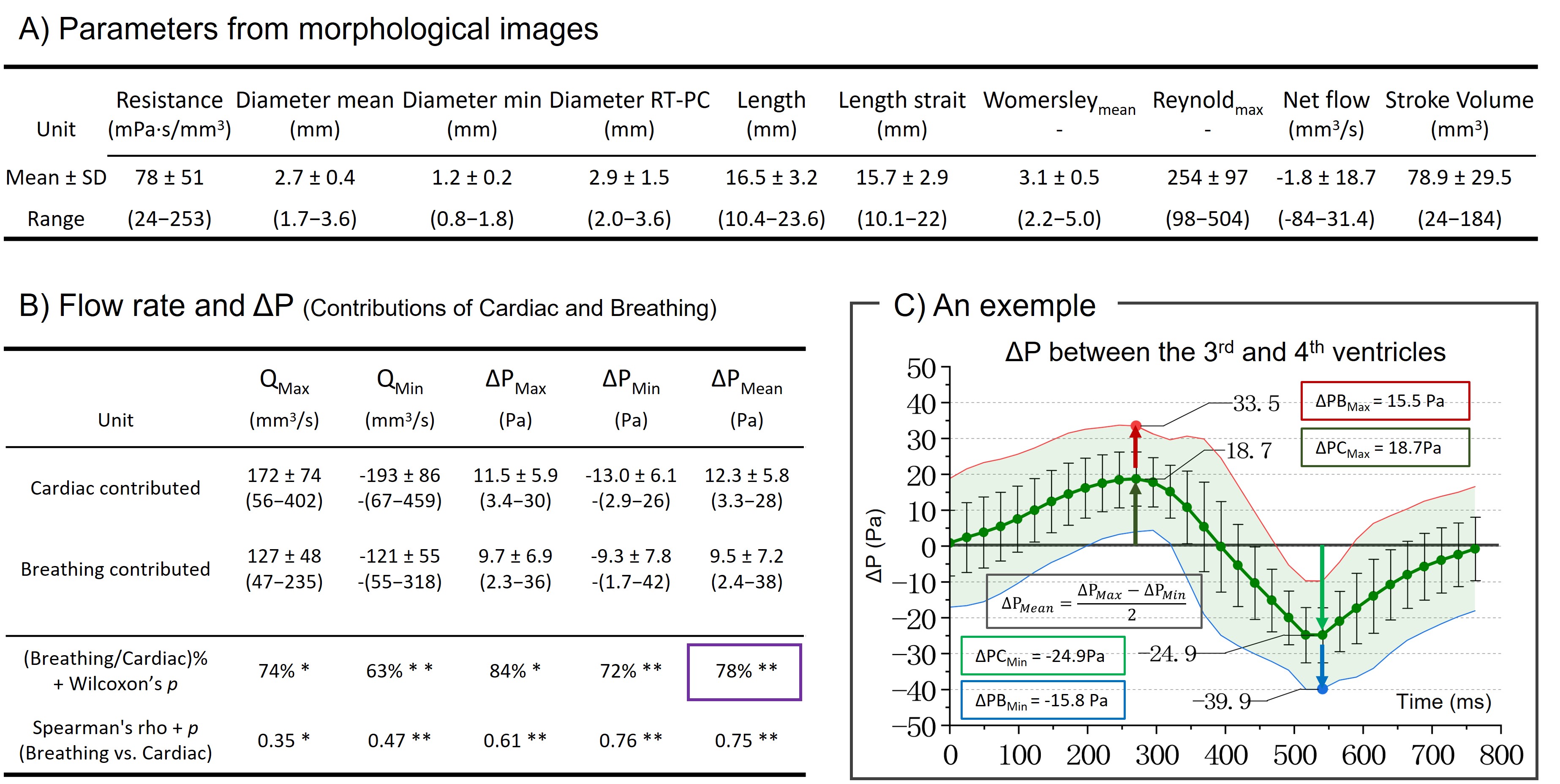
The ΔP was calculated by multiplying the obtained R with Q, representing the pressure difference between the fourth and third ventricles.
Results
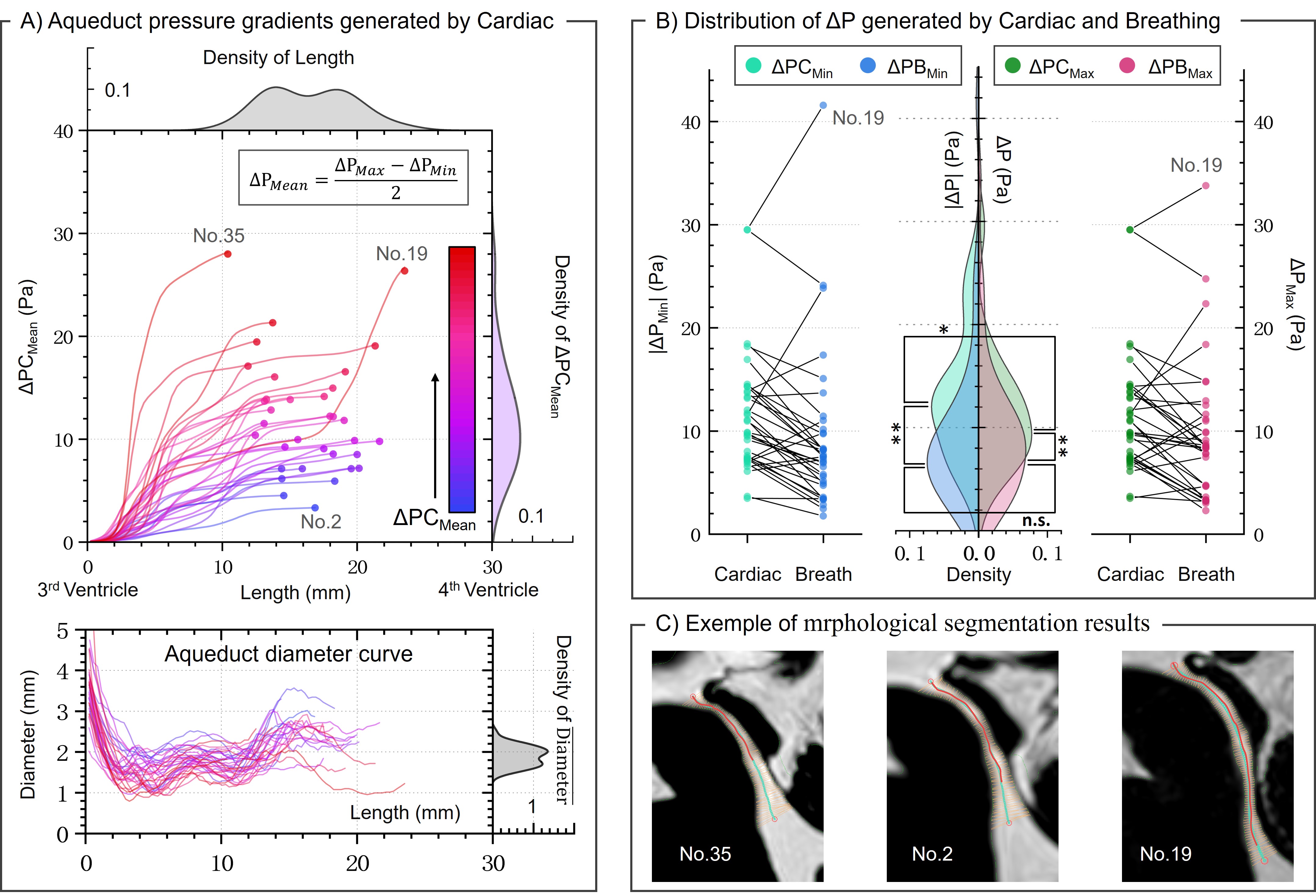
Fig.3 shows that the CSF Reynolds number is below 2000, consistent with laminar flow characteristics; the mean Womersley number is 3. ΔPCMean was equal to 12.3±5.8 Pa, whereas ΔPBMean was equal to 9.5±7.2 Pa. ΔPBC was equal to 78%.Fig.4 illustrates the variation curve of the pressure gradient through the aqueduct, using ΔPCMean as an example. Fig.4-B shows that |ΔPCMin| > ΔPCMax, while ΔPBMax is not significantly different from ΔPBMin.
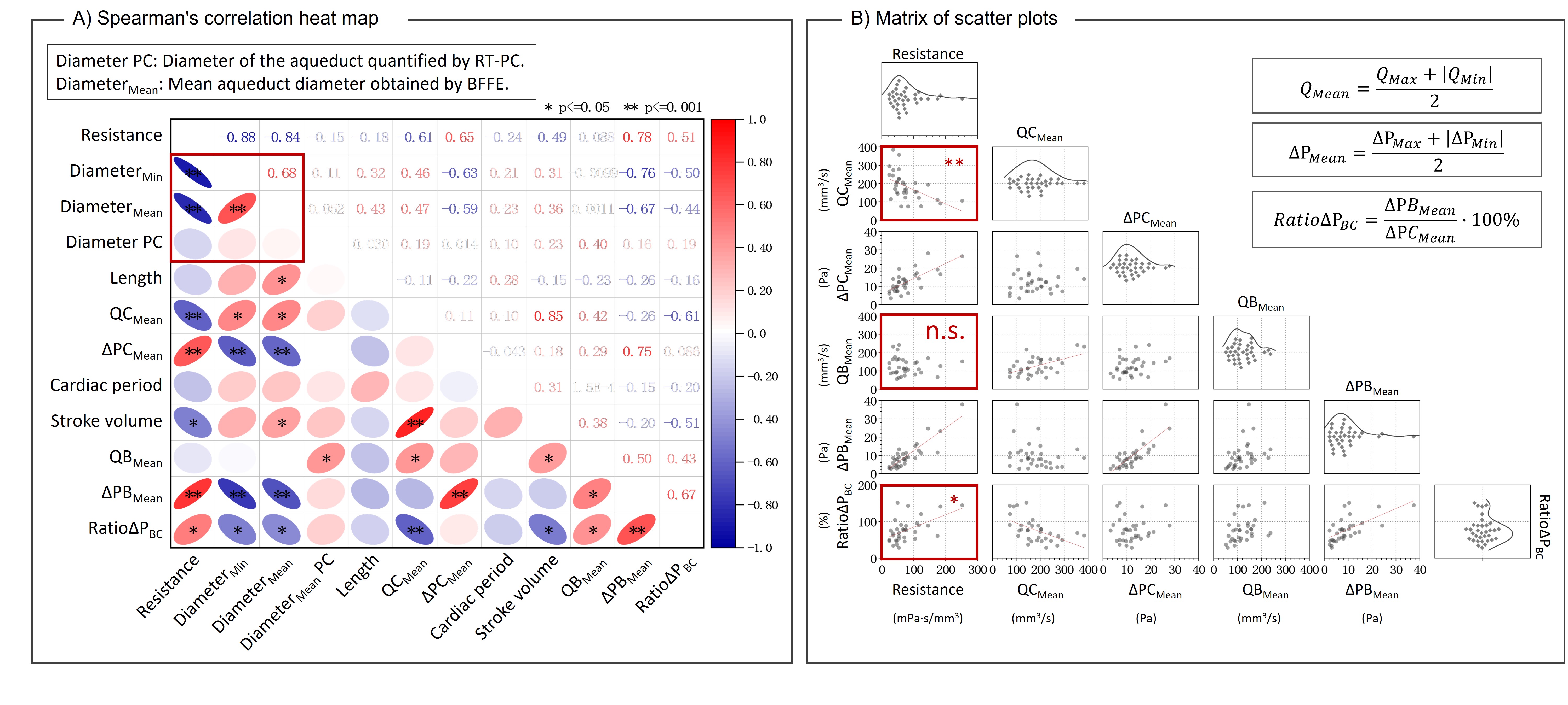
No correlation was observed between the aqueduct diameters obtained from RT-PC and BFFE (Fig.5-A). Instead,resistance correlates with RatioΔPBC. Analysis of Fig.5-B reveals a negative correlation of resistance with QCMean and no correlation with QBMean, suggesting that resistance affects flow from cardiac sources but not from respiratory sources.
Discussion
Finite element segmentation of aqueduct morphology is crucial for accurately quantifying interventricular pressure. This platform streamlines the process and improves the accuracy of quantification. Future analysis of dynamic effects using Navier-Stokes equations11 is also possible due to its high scalability.The breathing effect plays a significant role in quantifying the interventricular pressure difference, accounting for 78% of the cardiac-induced ΔP. Breathing-driven flow (QB) appears to be unaffected by changes in resistance, suggesting a decoupling from low-frequency respiratory influences, which is interesting to investigate. Breath-induced pressure changes may have significant clinical potential.
Conclusion
By combining anatomical MRI imaging with real-time phase-contrast MRI, it is possible to quantify the pressure difference between the third and fourth ventricles (ΔP) that drives CSF oscillations in the aqueduct. We have developed dedicated software for this purpose. Using continuous temporal acquisition of CSF flows in young healthy populations, we defined a reference physiological ΔP. We also quantified how cardiac and breathing functions influence this pressure. Such studies could contribute to a better understanding of the physiopathology of idiopathic hydrocephalus and hypertensive disorders.Acknowledgements
This research was supported by EquipEX FIGURES (Facing Faces Institute Guilding Research), Hanuman ANR-18-CE45-0014 and Region Haut de France. Thanks to the staff members at the Facing Faces Institute (Amiens, France) for technical assistance. Thanks to David Chechin from Phillips industry for his scientific support.References
1. Sincomb S, Coenen W, Sánchez AL, Lasheras JC. A model for the oscillatory flow in the cerebral aqueduct. Journal of Fluid Mechanics. 2020 Sep;899:R1. https://doi.org/10.1017/jfm.2020.463.2. Sincomb S, Moral-Pulido F, Campos O, Martinez-Bazan C, Haughton V, Sánchez AL. An In-Vitro Experimental Investigation of Oscillatory Flow in the Cerebral Aqueduct. Research Square. 2023 Apr 3. https://doi.org/10.2139/ssrn.4564789.
3. Bardan G, Plouraboué F, Zagzoule M, Balédent O. Simple patient-based transmantle pressure and shear estimate from cine phase-contrast MRI in cerebral aqueduct. IEEE transactions on biomedical engineering. 2012 Aug 8;59(10):2874-83.
4. Markenroth Bloch K, Töger J, Ståhlberg F. Investigation of cerebrospinal fluid flow in the cerebral aqueduct using high-resolution phase contrast measurements at 7T MRI. Acta Radiologica. 2018 Aug;59(8):988-96.
5. Liu P, Fall S, Ahiatsi M, Balédent O. Real-time phase contrast MRI versus conventional phase contrast MRI at different spatial resolutions and velocity encodings. Clinical Imaging. 2023 Feb 1;94:93-102. https://doi.org/10.1016/j.clinimag.2022.11.015.
6. Chen L, Beckett A, Verma A, Feinberg DA. Dynamics of respiratory and cardiac CSF motion revealed with real-time simultaneous multi-slice EPI velocity phase contrast imaging. Neuroimage. 2015 Nov 15;122:281-7. https://doi.org/10.1016/j.neuroimage.2015.07.073.
7. Fin L, Grebe R. Three dimensional modeling of the cerebrospinal fluid dynamics and brain interactions in the aqueduct of sylvius. Computer methods in biomechanics and biomedical engineering. 2003 Jun 1;6(3):163-70. https://doi.org/10.1080/1025584031000097933
8. Liu P, Lokossou A, Fall S, Makki M and Bamendent O, 2019. Post Processing Software for Echo Planar Imaging Phase Contrast Sequence. ISMRM 27th, (4823). https://archive.ismrm.org/2019/4823.html
9. Balédent O, Idy-peretti I. Cerebrospinal fluid dynamics and relation with blood flow: a magnetic resonance study with semiautomated cerebrospinal fluid segmentation. Investigative radiology. 2001 Jul 1;36(7):368-77.
10. Liu P, Fall S, Balédent O. Flow 2.0-a flexible, scalable, cross-platform post-processing software for realtime phase contrast sequences. In ISMRM 2022-International Society for Magnetic Resonance in Medicine 2022 May 7. https://archive.ismrm.org/2022/2772.html
11. Jacobson EE, Fletcher DF, Morgan MK, Johnston IH. Fluid dynamics of the cerebral aqueduct. Pediatric neurosurgery. 1996 Mar 7;24(5):229-36. https://doi.org/10.1159/000121044
Figures