1186
Monitoring pulsatile CSF motion in the subarachnoid space using MRI1Department of Biomedical Engineering, Johns Hopkins University School of Medicine, Baltimore, MD, United States, 2Department of Radiology, Johns Hopkins University School of Medicine, Baltimore, MD, United States, 3F.M. Kirby Research Center for Functional Brain Imaging, Kennedy Krieger Research Institute, Baltimore, MD, United States
Synopsis
Keywords: Neurofluids, Neurofluids
Motivation: The characterization of pulsatile cerebrospinal fluid (CSF) flow within the subarachnoid space remains insufficiently understood, presenting a challenge in distinguishing CSF flow from blood flow.
Goal(s): Our goal was to develop a time-efficient approach to monitor pulsatile CSF motion, independent of the pulsatile blood signal.
Approach: We introduced a cardiac-gated BOLD sequence with flow-sensitive bipolar gradients to characterize CSF motion, and evaluated blood contamination using cardiac-gated arterial-spin-labeling.
Results: We demonstrated that the main cause of the signal fluctuation is pulsatile CSF. The fluctuation patterns could be characterized by two components (hump and trough), which were consistently observe across subjects.
Impact: The pulsatile CSF motion in the subarachnoid space can now be efficiently monitored with our method. This technique complements the ventricular CSF motion methods and together they may provide a better understanding of CSF and glymphatic circulation in the brain.
INTRODUCTION
Cerebrospinal fluid (CSF) plays an important role in the brain’s waste clearance system.1,2 While CSF flow in the ventricles has been extensively studied, primarily using flow-sensitive techniques such as phase-contrast MRI,3-5 its flow in the subarachnoid space is poorly characterized. One of the challenges is that CSF flow in the subarachnoid space does not follow a known conduit, thus velocity mapping is less straightforward. The other challenge is that it is difficult to differentiate CSF flow from blood flow. Here we demonstrate that a cardiac-gated BOLD EPI acquisition with optimally weighted flow-sensitization gradients can provide a highly efficient approach to monitor pulsatile CSF motion, independent of the pulsatile blood signal. This sequence takes only 5 minutes and provides whole-brain coverage, making it highly practical in future clinical applications.METHODS
Experiment 1: Proof of the principle: The sequence used in this study is a multi-slice gradient-echo (GRE) BOLD sequence with a flow-sensitive bipolar gradient placed before the EPI acquisition6 (Figure 1a). Cardiac gating was recorded simultaneously with the MRI acquisition using a pulse device, allowing retrospective sorting of the images based on their cardiac phases. In Experiment 1, four encoding velocities along the foot-to-head direction were tested (VENC=0.4, 1, 4cm/s and infinity). Four healthy subjects (25.0±4.7 years) were scanned on a 3T Siemens Prisma system. Imaging parameters are: FOV=220×220×98.8mm³, voxel-size=3.44×3.44×3.8mm³, TR/TE=1550/36.0ms, number-of-dynamics=200, scan time 5’21”.Experiment 2: Confirmation that the signal source is CSF, not blood: The signal fluctuation over the cardiac cycle observed in Experiment 1 can be due to two main sources: 1) arterial blood, and 2) CSF in the subarachnoid space. To confirm that the signal we saw was not due to blood pulsation, we conducted a cardiac-gated multi-slice pseudo-continuous arterial spin labeling (pCASL) MRI. A minimal post-labeling delay of 1.39ms (not seconds) was used to ensure that the labeled blood was measured within the arteries. A bipolar gradient (VENC=1, 4cm/s) was applied before the EPI acquisition, similar to the setting in Experiment 1. Other imaging parameters were: labeling duration=2500ms, voxel size=3.44×3.44×5mm³, TR/TE=2960/27.0ms, number-of-pairs = 60.
RESULTS AND DISCUSSION
Figure 1c displays the dependence of the GRE signal on cardiac phase in an ROI around posterior cerebral artery (PCA) (Figure 1b) in 4 subjects. It can be seen that the VENC=inf data showed little fluctuation with cardiac phase. As VENC decreases, there is a reduction in signal amplitude across the cardiac phases. This presumably is due to the blood signal being suppressed. On the other hand, the cardiac-phase-dependent fluctuations also become apparent. In these data, the most pronounced signal fluctuation was observed when VENC=0.4 cm/s, with a fluctuation amplitude of 13%~50%. Moreover, the fluctuation timing/patterns were consistent across subjects.To confirm that these fluctuations are not due to blood, we used ASL in which the signs of the blood magnetization should be opposite between control and labeled images. Figure 2a shows the CBF maps acquired from pCASL, which is not the primary interest of this work. Figure 2b shows the control and labeled signals as a function of cardiac phase. Notice that the control and labeled signals revealed the same temporal pattern, not opposite, suggesting that the signal fluctuations we observed were not due to blood signals.
Recognizing that the fluctuation pattern consists of two components, a positive hump and a negative trough, we divided the signals (Figure 3a) into two kernels (Figures 3b). We then conducted a voxel-by-voxel fitting to determine the amplitude of each component, resulting in two maps. Figure 3c shows maps from a representative subject. It can be seen that, compared to static tissue, the signal fluctuations are more pronounced in the CSF-rich space, for example around the circle of Willis and in the Sylvian fissure. Interestingly, the two components contributed differently in different regions. For instance, the signal around PCA exhibited both hump and trough, while the signal around the Sylvian fissure tends to exhibit a trough-only pattern (Figure 3d). This heterogeneity can be potentially attributed to the compartmentalization of CSF around the brain, resulting in different pulsation patterns.
To test the reproducibility of the maps, Figure 4a shows maps of two runs in one representative subject. The scatter plots between the two runs are shown in Figure 4b. The spatial correlations (R1=0.92±0.04, R2=0.99±0.006, Figure 4c) suggests an outstanding reproducibility.
CONCLUSION
We demonstrated a time-efficient technique to monitor the pulsatile CSF motion in the subarachnoid space. This technique complements the ventricular CSF motion methods and together they may provide a better understanding of CSF and glymphatic circulation in the brain.Acknowledgements
No acknowledgement found.References
1. Taoka T, Naganawa S. Glymphatic imaging using MRI. J Magn Reson Imaging 2020;51:11-24.
2. Jiang Q. MRI and glymphatic system. Stroke Vasc Neurol 2019;4:75-77.
3. Markenroth Bloch K, Toger J, Stahlberg F. Investigation of cerebrospinal fluid flow in the cerebral aqueduct using high-resolution phase contrast measurements at 7T MRI. Acta Radiol 2018;59:988-996.
4. Dong Z, Wang F, Strom AK, Eckstein K, Bachrata B, Robinson S, Rosen B, Wald LL, Lewis LD, Polimeni JR. 4D CSF flowmetry to map brain-wide slow CSF flow dynamics and patterns in subarachnoid space. In: Proceedings of the ISMRM & SMRT Annual Meeting & Exhibition 32th Annual Meeting. 2023.
5. Chen L, Beckett A, Verma A, Feinberg DA. Dynamics of respiratory and cardiac CSF motion revealed with real-time simultaneous multi-slice EPI velocity phase contrast imaging. Neuroimage 2015;122:281-287.
6. Cao Y, Fan H, Xu C, Lu H. Toward vessel-suppressed cerebrovascular reactivity (CVR) mapping by using crusher gradients. In: Proceedings of the ISMRM & SMRT Annual Meeting & Exhibition 32th Annual Meeting. 2023.
Figures
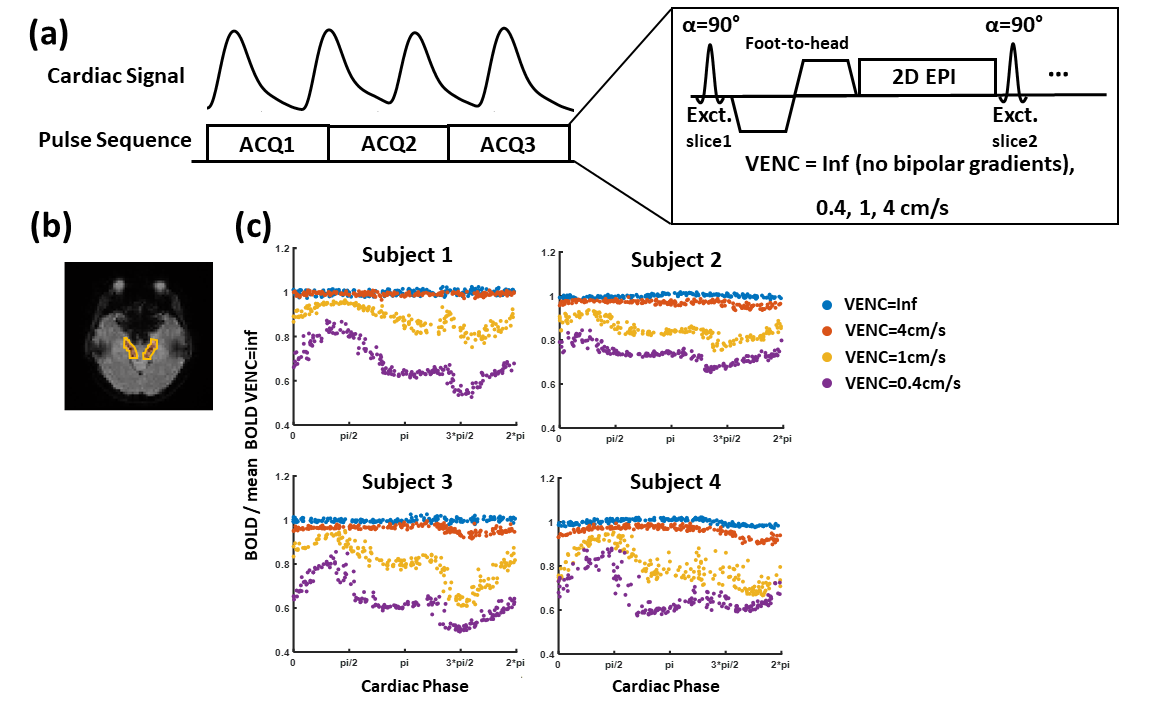
Figure 1. Pulse sequence diagram and representative data. (a) Sequence diagram of the multi-slice gradient-echo BOLD sequence with flow-sensitive gradients. Cardiac gating was recorded simultaneously with the MRI acquisition using a pulse device, allowing retrospective sorting of the images based on their cardiac phases. (b) Illustration or region of interest (ROI) around the posterior cerebral artery. (c) The dependence of the GRE signal on cardiac phase within ROI in 4 subjects. Signals were normalized by the temporal mean of signal with VENC=Inf.
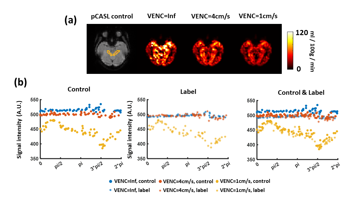
Figure 2. Cardiac-gated multi-slice pCASL data of a representative. (a) pCASL control image and CBF maps with VENC=Inf, VENC=4cm/s and VENC=1cm/s. (b) The dependence of pCASL control/label signal on cardiac phase.
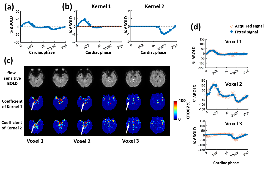
Figure 3. Mapping of the hump component and trough component of the pulsatile CSF. (a) Subject-specific signal around the posterior cerebral artery. (b) Two kernels obtained by dividing the signal in (a). Kernel 1 represents the hump component of the pulsatile signal, and kernel 2 represents the trough component. (c) Voxel-by-voxel fitting map of the two kernels of a representative subject, representing the amplitudes of hump/trough components. (d) Comparison between the fitted signal and the acquired signal in 3 representative voxels.
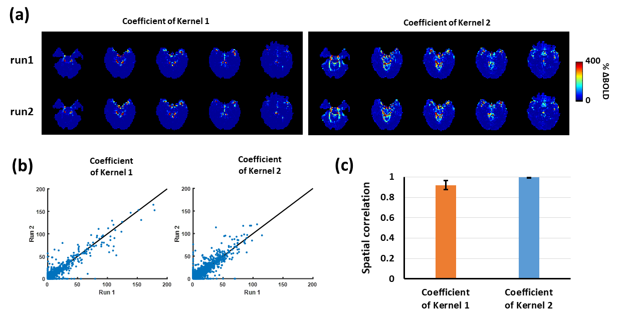
Figure 4. Test-retest reproducibility of map fitting of the hump/trough components. (a) Fitted coefficient maps of kernel 1 and kernel 2 of a representative using the BOLD data from 2 runs. (b) Scatter plots of coefficients of kernel 1 and kernel 2 obtained from two runs. (c) Spatial correlation between the coefficient maps of two runs in 4 healthy subjects.