0886
Characterizing spatial heterogeneity of BOLD fMRI cortical-depth profiles of activation: the average profile may not be typical1Athinoula A. Martinos Center for Biomedical Imaging, Massachusetts General Hospital, Charlestown, MA, United States, 2Department of Radiology, Harvard Medical School, Boston, MA, United States, 3Harvard-MIT Division of Health Sciences and Technology, Massachusetts Institute of Technology, Cambridge, MA, United States
Synopsis
Keywords: fMRI Analysis, fMRI, fMRI Analysis, fMRI (task based), Brain, Gray Matter, Neuroscience, Blood, Data Analysis
Motivation: Laminar-fMRI analysis routinely averages cortical-depth profiles within an ROI to estimate a typical laminar activation profile and increase SNR. Previous studies suggested heterogeneity of cortical-depth profiles measured with GE-BOLD-fMRI, therefore the assumption that profiles inside ROI are similar may not hold.
Goal(s): To test whether the average cortical-depth profile is typical for the whole ROI.
Approach: We applied k-means clustering to identify cortical locations within an ROI with similar BOLD-fMRI cortical-depth profiles.
Results: Cortical-depth profiles vary substantially across the activated region and therefore the average response profile inside the ROI may not be resemble that of any particular activated location.
Impact: In laminar-fMRI analysis, due to heterogeneity of neuronal responses and/or vascular architecture the average cortical-depth profile within an ROI may not match the profile at any one location, suggesting that averaging may lose meaningful layer-specific information within the activated region.
Introduction
Sub-millimeter-resolution laminar-fMRI studies typically summarize activation across cortical depths by generating cortical-depth profiles averaged over a specific region-of-interest (ROI) in the targeted cortical area. This pooling of laminar-fMRI data reduces biases associated with sampling some depths more than others1,2 and increases SNR, thus enabling small-voxel laminar-fMRI experiments even at lower (e.g., 1.5T) magnetic field strengths3, and the use of fMRI contrasts with higher spatial specificity but lower functional sensitivity than BOLD4. However, this anatomically-informed spatial averaging approach assumes similar cortical-depth profiles at each location within the ROI, except for spatially uncorrelated noise. This may not be the case. Earlier studies suggested that there may be substantial and perhaps meaningful heterogeneity of cortical-depth profiles generated from gradient-echo BOLD even within a small ROI5–7, with the highest spatial variability seen near the pial-surface5. We previously applied k-means spatial clustering to BOLD fMRI data to identify locations with similar temporal evolutions of cortical depth-dependent responses to visual-stimuli8, and the resulting spatial clusters exhibited cortical-depth profiles that differed from the average cortical-depth profile from the ROI. Here we extend this work by focusing on a single post-stimulus time-point to address the question: is the average cortical-depth profile typical for the whole ROI?Methods
Six healthy volunteers (3M/3F, 28±8y.o.) provided written informed consent before scanning, following our institution’s Human Subjects Research Committee policies. Imaging was performed on a whole-body 7T scanner (Terra, Siemens Healthineers, Erlangen, Germany) with an inhouse-built 64-channel receive-coil-array9. fMRI consisted of 10 runs per session of 2D-gradient-echo BOLD-weighted EPI with 0.8-mm isotropic-resolution8, coronally-oriented and positioned on the calcarine sulcus. During each run subjects were presented with a visual-stimulus: a flickering ’scaled-black-and-white-noise’ pattern in four randomly-jittered 16-s blocks and 40–49-s inter-stimulus-intervals. Same-session 0.75-mm isotropic-resolution FOCI-MEMPRAGE10,11 and a B0 field-map were also acquired.The T1 data were bias-field corrected (SPM) and FreeSurfer surface-meshes were reconstructed every 10% between WM and pial-surface2. EPI data were motion-corrected (AFNI), detrended and used to create dynamic-statistical-parameter-maps (dSPM)12. dSPM maps were averaged across runs and projected onto the surface-meshes following boundary-based registration13. GLM analyses performed in volume-space (FSL) yielded z-statistic maps which were combined across all runs using a fixed-effect analysis and projected onto the cortical surface-meshes to create activated region-of-interest (ROI) for each hemisphere.For each subject, k-means clustering (k=4) was applied to cortical-depth profiles of dSPM (t-statistic) from all surface-mesh vertices within the ROI (hemispheres combined) at a selected post-stimulus time-point (8 or 16s) and response-profiles inside each cluster were plotted.
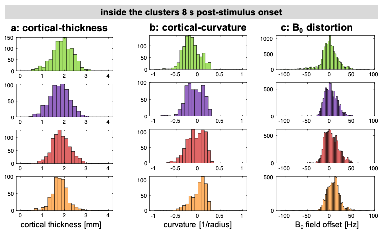
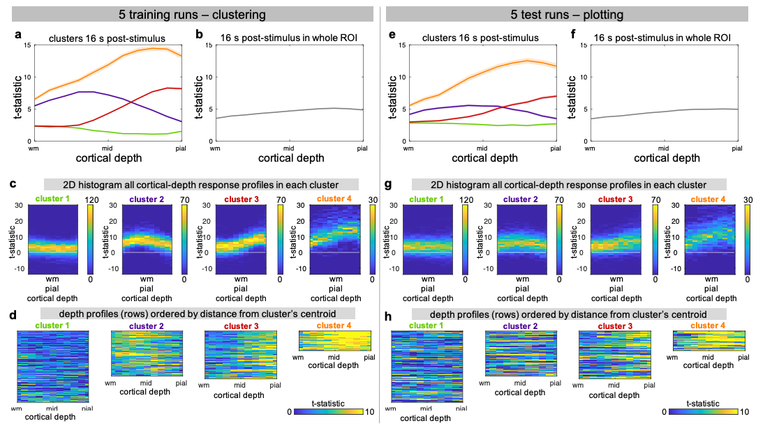
To test for systematic relationships between cortical features/artefacts and cluster membership, histograms of cortical-thickness, cortical-curvature and B0 field offsets inside the clusters were generated. Intra-subject train-test validation was performed: dSPM profiles averaged for five out of ten randomly-selected runs were clustered and response-profiles within these clusters were plotted.
To test whether similar clusters would be found by clustering noise, a synthetic-noise dataset distribution-matched to the dSPM map of an example subject was clustered following identical procedures as for the activation data. Finally, 10 synthetic-noise datasets were generated matching the data of 10 fMRI runs, then corrected with motion-estimates from the corresponding runs and clustered.
Results
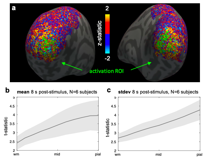
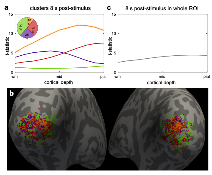
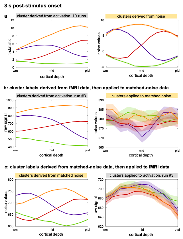
We observed spatial heterogeneity of cortical-depth profiles of BOLD activation (Figure 1); indeed, the cluster profiles differed from the average profile (Figure 2). Cortical-thickness, cortical-curvature and local distortions were similar within the four clusters, indicating that clustering is not driven/biased by these features (Figure 3). Intra-subject consistency of the clusters was confirmed using train-and-test approach on random subsets of runs (Figure 4). We found that the clustering algorithm yields plausible cortical-depth profiles when applied to synthetic-noise (Figure 5), indicating caution should be exercised. However, the noise-derived clusters yielded inconsistent cortical-depth profiles across runs whereas the activation-derived clusters were consistent (Figure 5b&c), demonstrating validity of activation-derived clustering of our data.Discussion
We have demonstrated that cortical-depth BOLD fMRI response-profiles vary substantially across the activated region. Pial vessels are sparse on the cortical surface14,15 which could contribute to spatial variation of the cortical-depth profiles – steeper near large veins6. Our results agree with a previous study where profile-sorting approach was used7. They are also consistent with reports demonstrating marked changes in cortical-depth profiles after excluding locations near large pial veins, which result in the peak BOLD activation-peak shifting from the pial-surface to mid-cortical depths16,17; if all cortical-depth profiles increased monotonically with depth like the average profile, this would not be observed. In conclusion, while using ROIs is necessary in laminar-fMRI analysis, the average cortical-depth profile within an ROI may not match the profile at any one location, suggesting that averaging may lose meaningful layer-specific information.Acknowledgements
We would like to thank Kyle Droppa for his help with subject recruitment and MRI scanning support, Azma Mareyam for 7T hardware support, and Dr. Saskia Bollmann for valuable discussions. This work was supported in part by the NIH NIBIB (grants P41-EB030006, R01-EB019437 and R01-EB032746), by the BRAIN Initiative (NIH NIMH grants R01-MH111419 and R00-MH120054, and by the MGH/HST Athinoula A. Martinos Center for Biomedical Imaging; and was made possible by the resources provided by NIH Shared Instrumentation Grants S10-OD023637 and S10-RR019371.References
1. Koopmans, P. J., Barth, M., Orzada, S. & Norris, D. G. Multi-echo fMRI of the cortical laminae in humans at 7 T. Neuroimage 56, 1276–1285 (2011).
2. Polimeni, J. R., Renvall, V., Zaretskaya, N. & Fischl, B. Analysis strategies for high-resolution UHF-fMRI data. Neuroimage 168, 296–320 (2018).
3. Markuerkiaga, I., Marques, J. P., Bains, L. J. & Norris, D. G. An in-vivo study of BOLD laminar responses as a function of echo time and static magnetic field strength. Sci. Rep. 11, 1–13 (2021).
4. Huber, L., Uludağ, K. & Möller, H. E. Non-BOLD contrast for laminar fMRI in humans: CBF, CBV, and CMRO2. Neuroimage 197, 742–760 (2019).
5. Polimeni, J. R., Fischl, B., Greve, D. N. & Wald, L. L. Laminar analysis of 7T BOLD using an imposed spatial activation pattern in human V1. Neuroimage 52, 1334–1346 (2010).
6. Gomez, D., Fultz, N., Polimeni, J. & Lewis, L. Temporal properties of fast BOLD fMRI responses in veins and parenchyma. in International Society for Magnetic Resonance in Medicine 2118 (2022).
7. Fracasso, A., Luijten, P. R., Dumoulin, S. O. & Petridou, N. Laminar imaging of positive and negative BOLD in human visual cortex at 7T. Neuroimage 164, 100–111 (2018).
8. Blazejewska, A. I., Gomez, D. & Polimeni, J. R. Temporal evolution of the cortical-depth profiles of BOLD fMRI response. in International Society for Magnetic Resonance in Medicine 4747 (2022).
9. Mareyam, A., Kirsch, J. E., Chang, Y., Madan, G. & Wald, L. L. A 64-Channel 7T array coil for accelerated brain MRI. in International Society for Magnetic Resonance in Medicine 0764 (2019).
10. Hurley, A. C. et al. Tailored RF Pulse for Magnetization Inversion at Ultrahigh Field. Magn. Reson. Med. 63, 51–58 (2010).
11. van der Kouwe, A. J. W., Benner, T., Salat, D. H. & Fischl, B. Brain morphometry with multiecho MPRAGE. Neuroimage 40, 559–569 (2008).
12. Dale, A. M. et al. Dynamic Statistical Parametric Mapping: Combining fMRI and MEG High-Resolution Imaging of Cortical Activity. Neuron 26, 55–67 (2000).
13. Greve, D. N. & Fischl, B. Accurate and robust brain image alignment using boundary-based registration. Neuroimage 48, 63–72 (2009).
14. Duvernoy, H. M., Delon, S. & Vannson, J. L. Cortical blood vessels of the human brain. Brain Res. Bull. 7, 519–579 (1981).
15. Bollmann, S. et al. Imaging of the pial arterial vasculature of the human brain in vivo using high-resolution 7T time-of-flight angiography. Elife 11, 1–35 (2022).
16. Koopmans, P. J., Barth, M. & Norris, D. G. Layer-specific BOLD activation in human V1. Hum. Brain Mapp. 31, 1297–1304 (2010).
17. Chen, G., Wang, F., Gore, J. C. & Roe, A. W. Layer-specific BOLD activation in awake monkey V1 revealed by ultra-high spatial resolution functional magnetic resonance imaging. Neuroimage 64, 147–155 (2013).
Figures