0813

Memory-efficient and robust model-based deep learning using non-montone monotone operator learning (MnM-MOL)

Maneesh John¹, Jyothi Rikhab Chand¹, and Mathews Jacob¹
¹Electrical and Computer Engineering, University of Iowa, Iowa City, IA, United States

Synopsis

Keywords: AI/ML Image Reconstruction, Machine Learning/Artificial Intelligence

Motivation: The high memory demand of model-based deep learning algorithms restricts their application in large-scale (eg., 3D/4D) applications. Moreover, their robustness to input perturbations is not well-studied.

Goal(s): To realize a memory efficient MoDL framework with similar theoretical guarantees as compressed sensing methods, while offering state-of-the-art performance.

Approach: We introduce a memory-efficient deep equilibrium framework with theoretical guarantees on uniqueness, convergence, and robustness.

Results: The proposed scheme offers comparable performance to state of the art methods, while being 10 times more memory-efficient. Additionally, the proposed scheme is significantly more robust to Gaussian and adversarial input perturbations.

Impact: The proposed approach results in greater than 10x reduction in memory demand, which enables the application of MoDL algorithms in large-scale (3D/4D) applications. The theoretically guaranteed robustness of the proposed algorithm reduces the error amplification in highly under-sampled settings.

Introduction

The recovery of MR images from undersampled measurements has been a topic of extensive research¹. Compressed sensing algorithms² have been shown to offer good performance, and additionally possess theoretical guarantees on uniqueness, convergence, and robustness to input perturbations. In recent years, several deep learning methods have been introduced^{3,4,5,6,7,8,9,10,11}. Unrolled model-based deep learning methods rely on iterative algorithms that alternate between data consistency steps and convolutional neural network (CNN) blocks. The network is unrolled for a small number of iterations, followed by end-to-end training of the CNN blocks⁶. While unrolled methods provide state-of-the-art performance, they require high GPU memory demand during training, restricting their utility to mostly 2D applications. In addition, the uniqueness of the solutions and robustness to perturbations in the measurements are not well-studied.

Deep equilibrium (DEQ) frameworks¹¹, such as monotone operator learning (MOL)¹², were recently introduced to reduce the high memory demand of unrolled algorithms. These methods use a single CNN block shared between iterations. When the Lipschitz constant of the CNN is less than one, the iterations converge to a fixed point¹¹. As DEQ methods use fixed point iterations rather than unrolling, they are very memory-efficient, requiring only a single physical block for both forward and backward propagation^11,12. However, the Lipschitz constraint on the CNN translates to reduced performance compared to unrolled methods¹².

Proposed approach

In this abstract, we introduce the following novel extensions to the MOL framework to relax the constraints on the CNN.

(a) Rather than constraining the CNN block $$$F_{\theta}$$$, we constrain the sum of the gradient of the data term and the CNN block $$Q_{\theta}(\mathbf x) = \mathbf A^H\mathbf A\mathbf x + \frac{1}{\lambda}F_{\theta}(\mathbf x)$$to be $$$m$$$-monotone. This extension is inspired by convex-non-convex methods^13,14, where a non-convex penalty is custom-designed with the data term so that the combined cost function is convex. This proposed approach allows the CNN to learn possibly non-monotone functions, thus improving performance.

(b) The monotone constraint is only imposed in a local region around the image manifold. In particular, we require $$$ Q_{\theta}= I- H_{\theta}$$$ to satisfy $$\max_{\mathbf z_1,\mathbf z_2\in B_{\delta}(\mathbf x)} \|H_{\theta}(\mathbf z_2)-H_{\theta}(\mathbf z_1)\| \leq (1-m)~\|\mathbf z_2-\mathbf z_1\|$$ for each training data point $$$\mathbf x$$$, where $$$B_{\delta}(\mathbf x)$$$ is a ball of radius $$$\delta$$$ centered at $$$\mathbf x$$$.

We propose the steepest descent algorithm $$\mathbf x_{k+1} = \mathbf x_k-Q_{\theta}(\mathbf x_k) + \mathbf A^H \mathbf b =H_{\theta}(\mathbf x_k) + \mathbf A^H \mathbf b \:\:\:\: (1).$$ to converge to the fixed points. With the above constraints, our theoretical results show that (a) the solution of (1) is unique within $$$B_{\delta}(\mathbf x)$$$, (b) the iterative algorithm will converge to the fixed points, and (c) the solution will be robust to input perturbations $$$\tilde{\mathbf b} = \mathbf b + \mathbf n$$$.

Experiments

We evaluate our approach using 2D multi-coil brain data from the publicly available Calgary-Campinas Public Dataset¹⁵. This dataset consists of T1-weighted brain scans from 117 healthy subjects, which were collected on a 3.0 Tesla MRI scanner. We selected a subset of 67 scans and divided them into 47 training and 20 testing sets.

We also used multichannel knee data from the fastMRI challenge¹⁶. This data set includes 15-coil coronal proton-density weighted knee images with or without fat suppression. We used the k-space measurements from 50 subjects for training, and 20 for testing.

Results

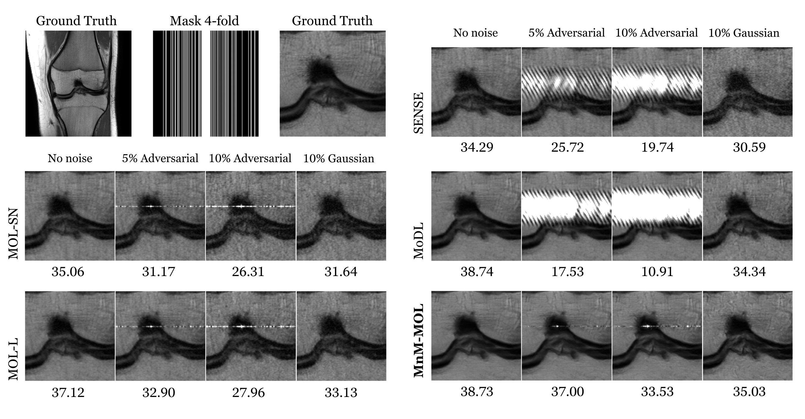
Figure 2 shows the results for four-fold accelerated brain data, and Figure 3 shows the results for four-fold accelerated knee data. MoDL offers the best PSNR and SSIM measures. The performance of MOL with spectral normalization (MOL-SN) is significantly worse than MoDL. Switching to a local monotone constraint (MOL-L) improves the performance, and the proposed MnM-MOL scheme offers further improvement. We attribute this improvement to (a) the non-monotone regularization prior, and (b) the local monotone constraint. The performance of MnM-MOL is only marginally lower than that of MoDL, but all of the MOL approaches use 10 times less memory than the unrolled MoDL approach. This improved memory efficiency would enable their application in larger-scale problems (e.g. 3D/4D).

Figure 4 and Figure 5 compare the robustness of these methods when Gaussian or worst-case adversarial noise is added to the input. We note that MoDL is significantly more robust to Gaussian noise than adversarial perturbation, and that a higher regularization parameter in SENSE would have resulted in a more robust approach at the expense of performance. Compared to MoDL and SENSE, all MOL approaches are more robust to both adversarial and Gaussian noise. We note that the proposed MnM-MOL scheme can maintain this robustness while also providing improved performance over MOL.

Acknowledgements

This work is supported by NIH grants R01-AG067078, R01-EB031169, and R01-EB019961.

References

1. J. A. Fessler, “Model-based image reconstruction for MRI,” IEEE signal processing magazine, vol. 27, no. 4, pp. 81–89, 2010.

2. M. Lustig, D. Donoho, and J. M. Pauly, “Sparse MRI: The application of compressed sensing for rapid MR imaging,” Magnetic Resonance in Medicine: An Official Journal of the International Society for Magnetic Resonance in Medicine, vol. 58, no.6, pp. 1182–1195, 2007.

3. K. Gregor and Y. LeCun, “Learning fast approximations of sparse coding,” in Proceedings of the 27th International Conference on Machine Learning, 2010, pp. 399–406.

4. Y. Romano, M. Elad, and P. Milanfar, “The little engine that could: Regularization by denoising (RED),” SIAM Journal on Imaging Sciences, vol.10, no. 4, pp. 1804–1844, 2017.

5. K. Hammernik et al., “Learning a variational network for reconstruction of accelerated MRI data,” Magnetic resonance in medicine, vol. 79, no. 6, pp. 3055–3071, 2018.

6. H. K. Aggarwal, M. P. Mani, and M. Jacob, “MoDL: Model-based deep learning architecture for inverse problems,” IEEE transactions on medicalimaging, vol. 38, no. 2, pp. 394–405, 2018.

7. Y. Sun, B. Wohlberg, and U. S. Kamilov, “An online plug-and-play algorithm for regularized image reconstruction,” IEEE Transactions on Computational Imaging, vol. 5, no. 3, pp. 395–408, 2019.

8. E. Ryu, J. Liu, S. Wang, X. Chen, Z. Wang, and W. Yin, “Plug-and-play methods provably converge with properly trained denoisers,” in International Conference on Machine Learning. PMLR, 2019, pp. 5546–5557.

9. Y. Sun, Z. Wu, X. Xu, B. Wohlberg, and U. S. Kamilov, “Scalable plug-and-play ADMM with convergence guarantees,” IEEE Transactions on Computational Imaging, vol. 7, pp. 849–863, 2021.

10. J. Xiang, Y. Dong, and Y. Yang, “FISTA-net: Learning a fast iterative shrinkage thresholding net-work for inverse problems in imaging,” IEEE Transactions on Medical Imaging, vol. 40, no. 5, pp. 1329–1339, 2021.

11. D. Gilton, G. Ongie, and R. Willett, “Deep equilibrium architectures for inverse problems in imaging,” IEEE Transactions on Computational Imaging, vol. 7, pp. 1123–1133, 2021.

12. A. Pramanik, M. B. Zimmerman, and M. Jacob, “Memory-efficient model-based deep learning with convergence and robustness guarantees,” IEEE Transactions on Computational Imaging, vol. 9, pp. 260–275, 2023.

13. A. Parekh and I. W. Selesnick, “Convex denoising using non-convex tight frame regularization,” IEEE Signal Processing Letters, vol. 22, no. 10, pp. 1786–1790, 2015.

14. A. Lanza, S. Morigi, I. W. Selesnick, and F. Sgallari, “Convex Non-convex Variational Models,” in Handbook of Mathematical Models and Algorithms in Computer Vision and Imaging. Springer, 2023.

15. R. Souza et al., “An open, multi-vendor, multi-field-strength brain MR dataset and analysis of publicly available skull stripping methods agreement,” NeuroImage, vol. 170, pp. 482–494, 2018.

16. J. Zbontar, F. Knoll, A. Sriram, T. Murrell, Z. Huang, M. J. Muckley, A. Defazio, R. Stern, P. Johnson, M. Bruno et al., “fastMRI: An open dataset and benchmarks for accelerated MRI,” arXiv preprint arXiv:1811.08839, 2018.

Figures

Figure 1: One step of the iterative steepest descent algorithm defined in (1). If the algorithm is initialized with $$$\mathbf x_0 \in \mathcal B_{\delta}(\mathbf x^*)$$$, the iterations are guaranteed to converge to a unique fixed point.

Figure 2: Reconstruction results of 4x accelerated Calgary brain data. The PSNR (dB) values for each case are reported. The image in the first row of the first column was undersampled using a Cartesian 2D nonuniform variable density mask, as seen in the second row of the first column. The upper row displays the reconstructions (magnitude images), while the lower row shows the corresponding error images.

Figure 3: Reconstruction results of 4x accelerated fastMRI knee data. The PSNR (dB) values for each case are reported. The image in the first row of the first column was undersampled using a Cartesian 1D nonuniform variable density mask, as seen in the second row of the first column. The upper row displays the reconstructions (magnitude images), while the lower row shows the corresponding error images.

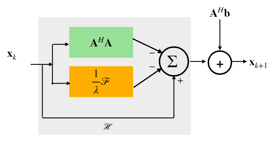
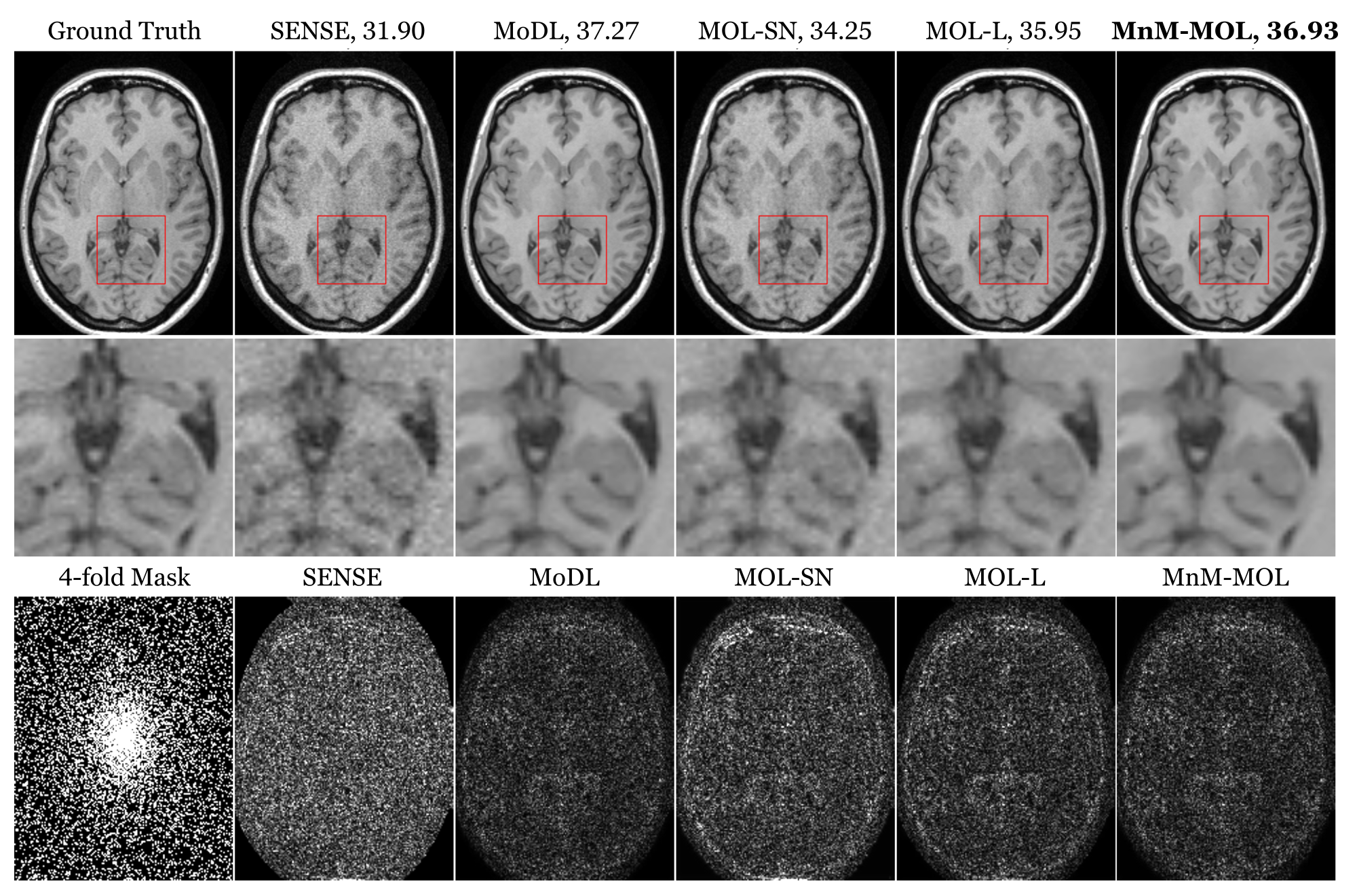
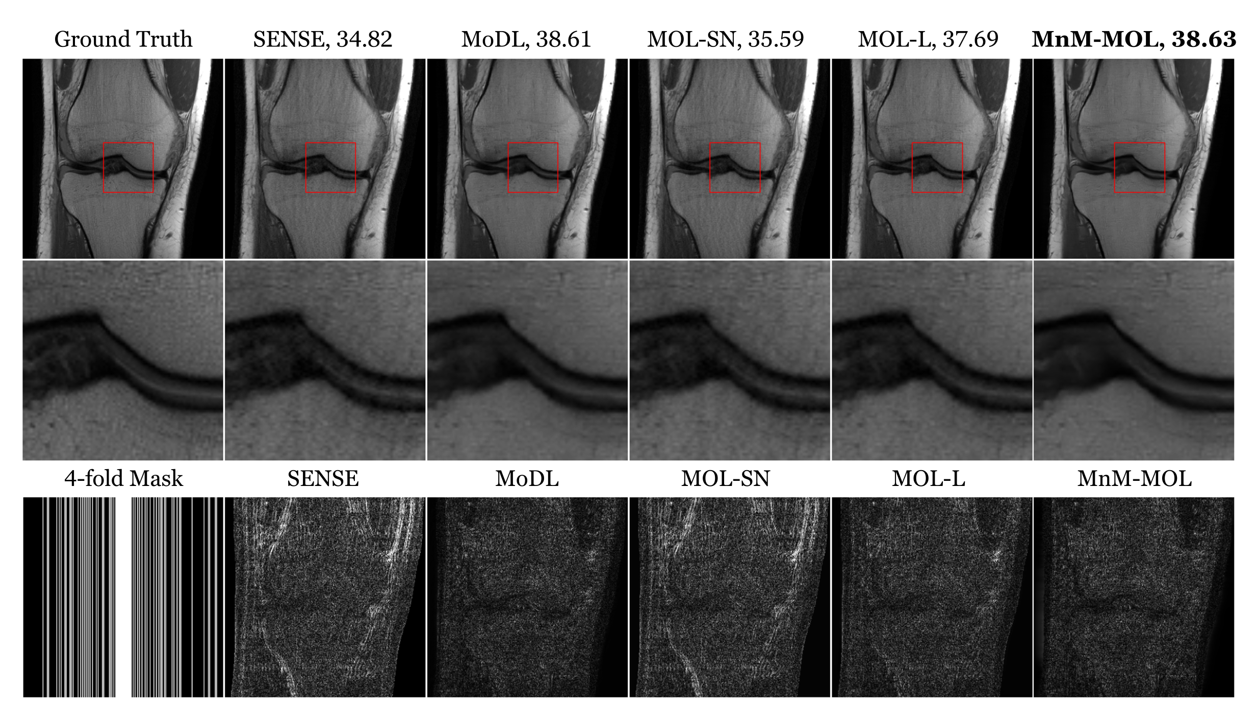
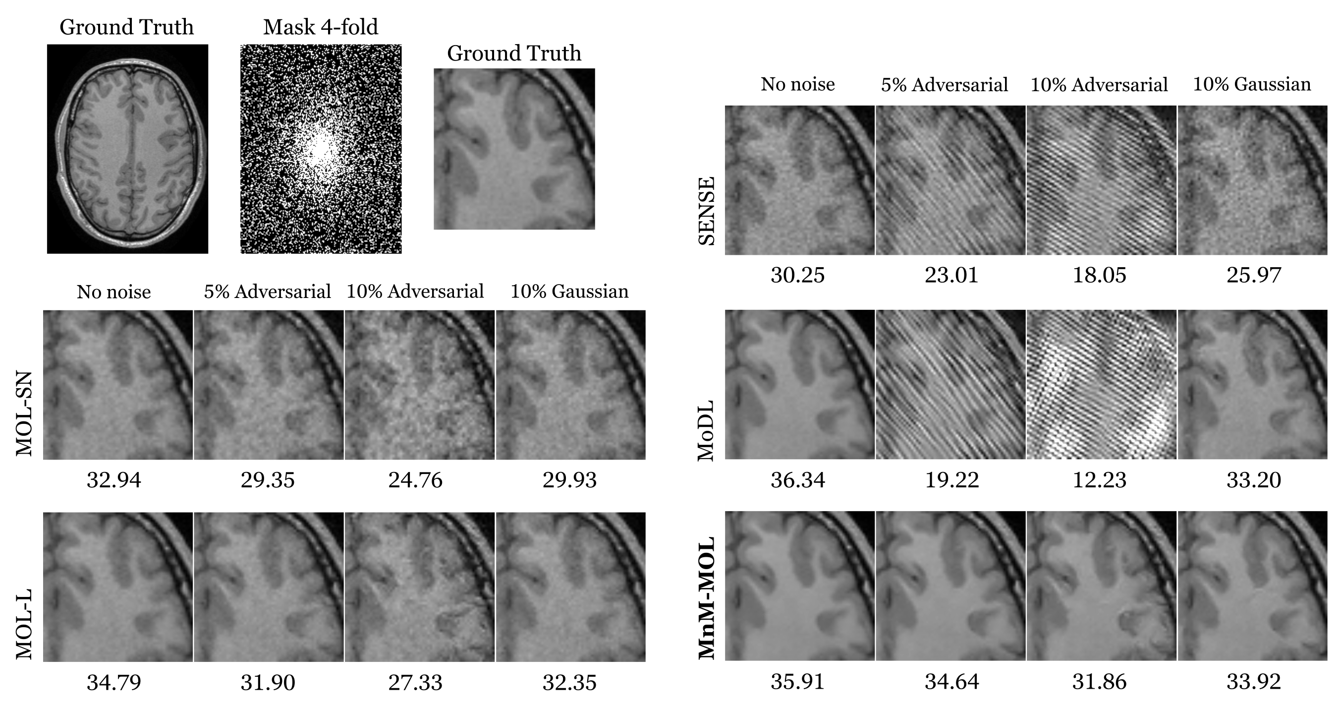
Figure 4: Sensitivity of the algorithms to input perturbations: The rows correspond to reconstructed images from 4x-accelerated Calgary brain data using different methods. The data was undersampled using a Cartesian 2D nonuniform variable density mask. The columns correspond to recovery without additional noise, worst-case added adversarial noise whose norm is 5% and 10% of the measured data, and Gaussian noise, whose norm is also 10% of the measured data, respectively. The PSNR (dB) values of the reconstructed images are reported for each case.

Figure 5: Sensitivity of the algorithms to input perturbations: The rows correspond to reconstructed images from 4x-accelerated fastMRI knee data using different methods. The data was undersampled along the phase-encoding direction using a Cartesian 1D nonuniform variable density mask. The columns correspond to recovery without noise, worst-case adversarial noise whose norm is 5% and 10% of the measured data, and Gaussian noise whose norm is also 10% of the measured data, respectively. The PSNR (dB) values of the reconstructed images are reported for each case.

Proc. Intl. Soc. Mag. Reson. Med. 32 (2024)

0813

DOI: https://doi.org/10.58530/2024/0813