0731
Hierarchical Bayesian Microstructure Modelling Improves Voxelwise Quantification of Blood-Brain Barrier Water Exchange Rates1Centre for Medical Image Computing, Medical Physics and Biomedical Engineering, University College London, London, United Kingdom, 2Queen Square MS Centre, Institute of Neurology, University College London, London, United Kingdom, 3Bioxydyn Limited, Manchester, United Kingdom, 4School of Computer Science and Informatics, Cardiff University, Cardiff, United Kingdom
Synopsis
Keywords: Blood Vessels, Neuro, blood-brain barrier
Motivation: Blood-brain barrier (BBB) water exchange (WEX) imaging techniques are increasingly used to quantify BBB dysfunction. However, WEX imaging is highly noise sensitive, which is typically addressed by averaging data spatially or across subjects.
Goal(s): To obtain robust, subject-specific, voxel-wise WEX quantification from BBB filter exchange imaging (FEXI) data.
Approach: We implement a hierarchical Bayesian model fitting method, which, by introducing a Gaussian prior for model parameters (estimated from the data), reduces sensitivity to voxel-wise noise.
Results: Relative to conventional least-squares estimation, Bayesian model fitting improves parameter estimation qualitatively and quantitatively in synthetic and in ten test-retest volunteer datasets.
Impact: Robust, subject-specific, voxel-wise WEX quantification from BBB filter exchange imaging (FEXI) data will enable localised BBB dysfunction to be identified in neurological disease, potentially enabling earlier diagnosis or discrimination between diseases.
Introduction
Microstructure modelling fits a mathematical model to acquired MRI data to estimate sub-voxel tissue features. Typically, feature maps are obtained by assuming independence between voxels and fitting the model voxel-by-voxel using least squares minimisation or machine learning; however, these approaches are sensitive to voxelwise noise, leading to potential errors in parameter estimation. Hierarchical Bayesian modelling can address this limitation by breaking the assumption of independent voxels with a prior distribution over model parameters across a region-of-interest (ROI). Crucially, the prior distribution is estimated from the data, along with the posterior distributions of voxelwise parameters, typically with Markov chain Monte Carlo (MCMC) methods. This ‘sharing’ of information across voxels improves fit stability; however, this approach has only been demonstrated for simple microstructure models such as IVIM1 or ball-and-stick2.Complex models, like those parameterising water exchange (WEX) rates across the blood-brain barrier (BBB), would benefit from Bayesian techniques: currently, WEX techniques are highly noise-sensitive, often requiring spatial or cross-subject data averaging. Here we utilise our recent generalised framework for Bayesian microstructure modelling2 and demonstrate it on synthetic and in vivo (test-restest) BBB filter exchange imaging (BBB-FEXI3) data.
Methods
Bayesian hierarchical modelFollowing Orton et al.1 we use a Bayesian hierarchical model:
$$p(\theta_{1:N},\mu,\Sigma|\textbf{y}_{1:N})\propto p(\textbf{y}_{1:N}|\theta_{1:M})p(\theta_i|\mu,\Sigma)p(\theta,\Sigma),$$
where $$$p(\theta_{1:N},\mu,\Sigma|\textbf{y}_{1:N})$$$ is the parameter posterior distribution for voxels 1..N, $$$p(\textbf{y}_{1:N}|\theta_{1:M})$$$ the likelihood, $$$p(\theta_i|\mu,\Sigma)$$$ the multivariate normal hierarchical prior, and $$$p(\theta,\Sigma)$$$ the prior. We estimate the parameter posterior and hierarchical prior distributions from the data. We use two extensions first introduced by Powell et al.2:
- Separate hierarchical priors for different ROIs, potentially more appropriate than a global prior for fitting across distinct neurological tissue types;
- Generalisation of the likelihood from Orton et al.1 to accommodate a versatile framework for any microstructure model.
Synthetic data
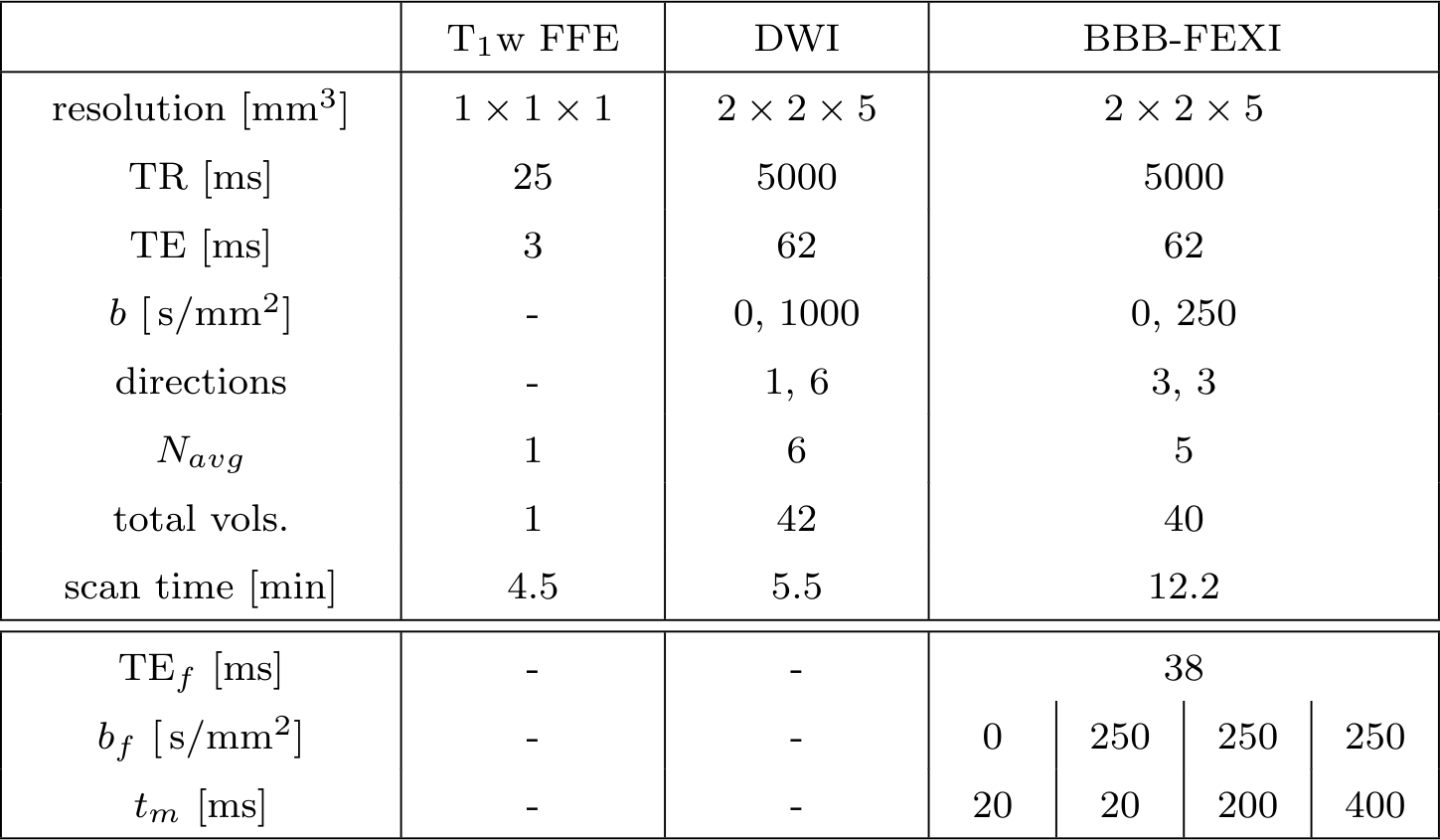
Signals (1225 voxels total) were simulated using the AXR model4,5 (acquisition scheme in Fig.1):
$$S = \exp\left(-ADC'\left(t_m\right)b\right),$$
where
$$ADC'\left(t_m\right)=ADC\left[1-\sigma\exp\left(-t_m\cdot AXR\right)\right],$$
with ADC and ADC'(tm) the apparent diffusion coefficients at equilibrium (i.e. filter inactive) and at each mixing time (tm) with the filter active, respectively, and σ the filter efficiency. Ground truth model parameters were normally distributed in two ROIs representative of WM/GM values3: (i) WM; ADC=0.90±0.04µm2/ms, σ=0.14±0.02, AXR=2.00±0.30s-1; (ii) GM; ADC=1.20±0.08µm2/ms, σ=0.18±0.03, AXR=1.40±0.35s-1. Zero-mean Gaussian noise was added to each signal to give SNR=100.
In vivo data
Ten healthy subjects (age range 23-52years; five female) were each scanned twice on a 3T Philips Ingenia CX system. Single slice BBB-FEXI data and whole brain DWI (for registration) and T1-weighted images (for WM/GM segmentation) were acquired (protocols and pre-processing in Fig.1).
Analysis
The AXR model (Eq.3) was fitted to all data (synthetic, in vivo) using least squares minimisation. The Bayesian model was fitted with MCMC2, using 1x10⁶ steps for each WM/GM ROI and initialised with the least squares-estimated values. Posterior distributions and representative statistics were generated for each parameter from samples after the burn-in period (5x10⁵steps).
Results
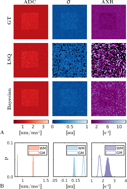
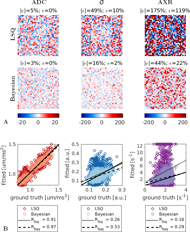
Synthetic dataFig.2 shows ground truth synthetic data, alongside parameter estimates obtained through least-squares and Bayesian methods (using mean values from the posterior distribution). Qualitatively, our Bayesian method performs better, with fewer extreme fits apparent; this is validated quantitatively by corresponding error maps in Fig.3, which also provide average and absolute percent errors.
In vivo data
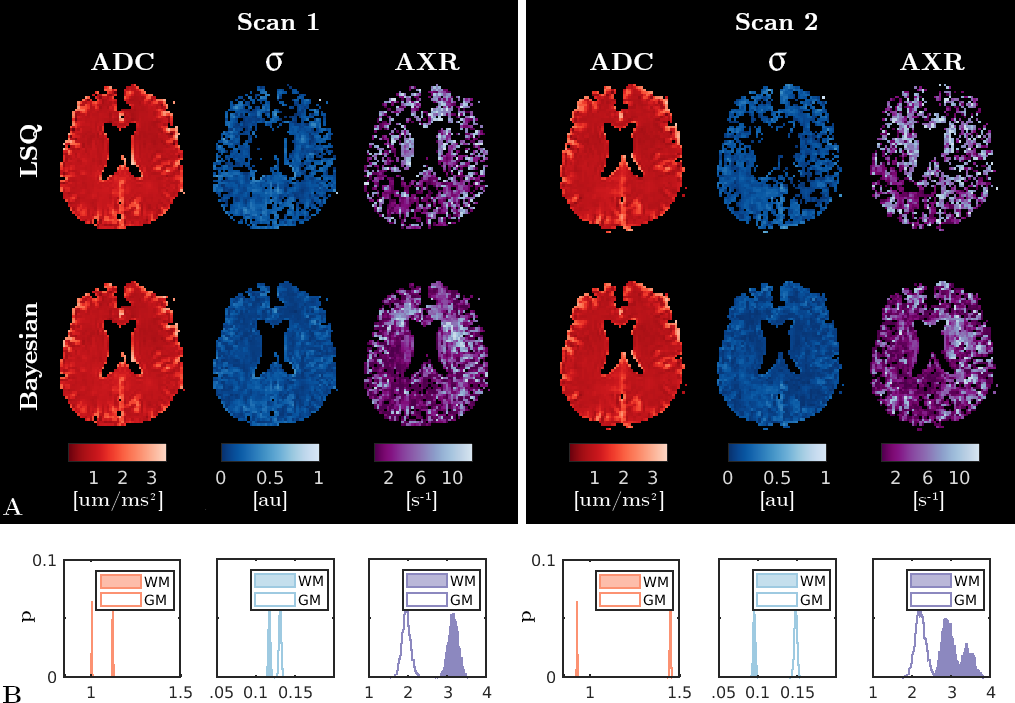
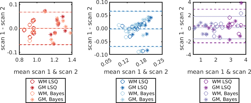
Fig.4 shows test-retest parameter maps from the least-squares and Bayesian estimation for an example subject. Qualitatively, our Bayesian method once again performs better, showing fewer extreme values. Bland-Altman plots are shown in Fig.5, where the 95% limits of agreement are improved (upper/lower limits reduced by 38%/28%, respectively) for Bayesian-fitted AXR values.
Discussion
The Bayesian fitting approach demonstrated substantially reduced errors in synthetic data (Fig.3), and better reconstructed the two distinct ROIs where noise levels in the least-squares estimation was too high to resolve them (Fig.2). This provides confidence that in vivo parameters estimated using Bayesian modelling are also more accurate (Fig.4).However, caution is needed in high noise situations, where the global prior may draw parameter values towards the mean of the constraints used during fitting, as opposed to the true parameter mean. Distinct WM/GM posterior distributions (Fig.4B) provide confidence we avoid this situation in vivo here.
Conclusions
BBB water exchange measurements, using metrics such as AXR, are highly sensitive to noise; we show here that Bayesian fitting can help reduce this sensitivity. In combination with other improvements - such as optimised acquisition protocols and advanced modelling incorporating relaxation effects3 - Bayesian fitting can contribute to the practical implementation of subject-specific, voxel-wise AXR estimation.Acknowledgements
This work was supported by EPSRC grants EP/S031510/1. Thanks to Dr David Higgins and Dr Matthew Clemence of Philips Healthcare MR Clinical Science for their support of this work.References
- M.R. Orton, D.J. Collins, D.M. Koh, and M.O. Leach. “Improved intravoxel incoherent motion analysis of diffusion weighted imaging by data driven Bayesian modeling”. In: Magnetic Resonance in Medicine 71.1 (2014), pp. 411–420. doi: 10.1002/mrm.24649.
- E. Powell, M. Battocchio, C.S. Parker, and P.J. Slator. “Generalised Hierarchical Bayesian Microstructure Modelling for Diffusion MRI”. In: Lecture Notes in Computer Science. Ed. by S. Cetin-Karayumak, D. Christiaens, M. Figini, P. Guevara, N. Gyori, V. Nath, and T. Pieciak. Vol. 13006 LNCS. Springer International Publishing, 2021, pp. 36–47. doi: 10.1007/978-3-030-87615-9_4.
- E. Powell, Y. Ohene, M. Battiston, B.R. Dickie, L.M. Parkes, and G.J.M. Parker. “Blood-brain barrier water exchange measurements using FEXI: Impact of modeling paradigm and relaxation time effects”. In: Magnetic Resonance in Medicine (2023). doi: 10.1002/mrm.29616.
- S. Lasic, M. Nilsson, J. Latt, F. Stahlberg, and D. Topgaard. “Apparent exchange rate mapping with diffusion MRI”. In: Magnetic Resonance in Medicine 66.2(2011), pp. 356–365. doi: 10.1002/mrm.22782.
- M. Nilsson, J. Latt, D. Van Westen, S. Brockstedt, S. Lasic, F. Stahlberg, and D. Topgaard. “Noninvasive mapping of water diffusional exchange in the human brain using filter-exchange imaging”. In: Magnetic Resonance in Medicine 69.6(2013), pp. 1573–1581. doi: 10.1002/mrm.24395.
- J.L.R. Andersson, S. Skare, and J. Ashburner. “How to correct susceptibility distortions in spin-echo echo-planar images: Application to diffusion tensor imaging”. In:NeuroImage 20.2 (2003), pp. 870–888.
- S.M. Smith, M. Jenkinson, M.W. Woolrich, C.F. Beckmann, T.E.J. Behrens, H. Johansen-Berg, P.R. Bannister, M. De Luca, I. Drobnjak, D.E. Flitney, R.K. Niazy, J. Saunders, J. Vickers, Y. Zhang, N. DeStefano, J.M. Brady, and P.M. Matthews. “Advances in functional and structural MR image analysis and implementation as FSL”. In: NeuroImage 23. (2004), pp. 208–219.5
- Y. Zhang, M. Brady, and S. Smith. “Segmentation of brain MR images through a hidden Markov random field model and the expectation-maximization algorithm”. In: IEEE Transactions on Medical Imaging 20.1 (2001), pp. 45–57.
- M. Jenkinson and S. Smith. “A global optimisation method for robust affine registration of brain images”. In: Medical Image Analysis 5.2 (2001), pp. 143–156.
Figures