0641

Cumulant tensors from the addition of angular momenta: All diffusion invariants in one abstract

Santiago Coelho^1,2, Filip Szczepankiewicz³, Els Fieremans^1,2, and Dmitry S Novikov^1,2
¹Bernard and Irene Schwartz Center for Biomedical Imaging, Department of Radiology, New York University Grossman School of Medicine, New York, NY, United States, ²Center for Advanced Imaging Innovation and Research (CAI2R), Department of Radiology, New York University Grossman School of Medicine, New York, NY, United States, ³Medical Radiation Physics, Clinical Sciences Lund, Lund University, Lund, Sweden

Synopsis

Keywords: Diffusion Modeling, Diffusion/other diffusion imaging techniques

Motivation: The advent of quantitative imaging hinges on revealing the information content of MRI measurements. We provide a complete basis- and hardware-independent “fingerprint" for the diffusion signal up to moderate diffusion-weightings.

Goal(s): Find all rotationally invariant information present in the cumulant expansion up to b².

Approach: We classify all invariants of diffusion and covariance tensors in terms of irreducible representations of the group of rotations, discuss their geometric meaning, and relate them to tissue properties.

Results: We find a complete set of 21 independent rotational invariants up to b². Previously studied contrasts are expressed via only 7, while the rest provide novel complementary information.

Impact: We map the diffusion covariance tensor onto the addition of angular momenta, and provide all rotational invariants of the cumulant expansion (RICE). RICE apply to >50k publicly available human diffusion MRI datasets, providing new insights into tissue properties.

Introduction

We know that the diffusion tensor¹ $$$\mathsf{D}_{ij}$$$ is an ellipsoid:
$$\mathsf{D}(\hat{\mathbf{n}})=\sum_{i,j}\mathsf{D}_{ij}n_in_j\equiv\mathsf{D}_{00}Y^{00}(\hat{\mathbf{n}})+\sum_m\mathsf{D}_{2m}Y^{2m}(\hat{\mathbf{n}}),\quad(1)$$
with isotropic part $$$\mathsf{D}_{00}\propto\mathrm{MD}$$$, and anisotropic part described by 5 spherical harmonic (SH) coefficients $$$\mathsf{D}_{2m}$$$ of degree $$$\ell=2$$$. Intuitively, $$$\ell=0\,\mathrm{(scalar)}$$$ and $$$\ell=2\,\mathrm{(tensor)}$$$ parts are different. This difference is formalized as follows: $$$\mathsf{D}_{\ell\,m}$$$ with different $$$\ell$$$ do not “mix” under rotations.

$$$\mathsf{D}$$$ has 3 rotational invariants $$$-$$$ quantities independent of the basis. The remaining 3 degrees of freedom (dof) define its orientation.

Our goal is to study the geometry of a more complex object $$$-$$$ the covariance tensor $$$\mathsf{C}_{ijkl}$$$ generalizing the kurtosis tensor² for arbitrary b-tensor encoding³,
$$\mathrm{ln}\,S=-\sum_{i,j}\mathsf{B}_{ij}\mathsf{D}_{ij}+\tfrac12\sum_{i,j,k,l}\mathsf{B}_{ij}\mathsf{B}_{kl}\mathsf{C}_{ijkl}+\mathcal{O}(b^3),\quad(2)$$
and relate it to tissue properties. We use the far-reaching decomposition (1) into irreducible components with different $$$\ell$$$, and construct all 18 independent invariants of $$$\mathsf{C}$$$. Together with $$$\mathsf{D}$$$, the 21 rotational invariants of the cumulant expansion (RICE) form the complete “fingerprint” of the dMRI signal up to $$$b^2$$$.
Remarkably, all previous model-independent contrasts (mean-radial-axial kurtosis²; isotropic-anisotropic variance^3,4) involve only 4 $$$\mathsf{C}$$$ invariants⁵. Together with 3 from $$$\mathsf{D}$$$, the 7 RICE invariants underpin any dMRI studies up to $$$b^2$$$. The remaining 14 invariants have not been systematically studied.

Covariance tensor from addition of angular momenta

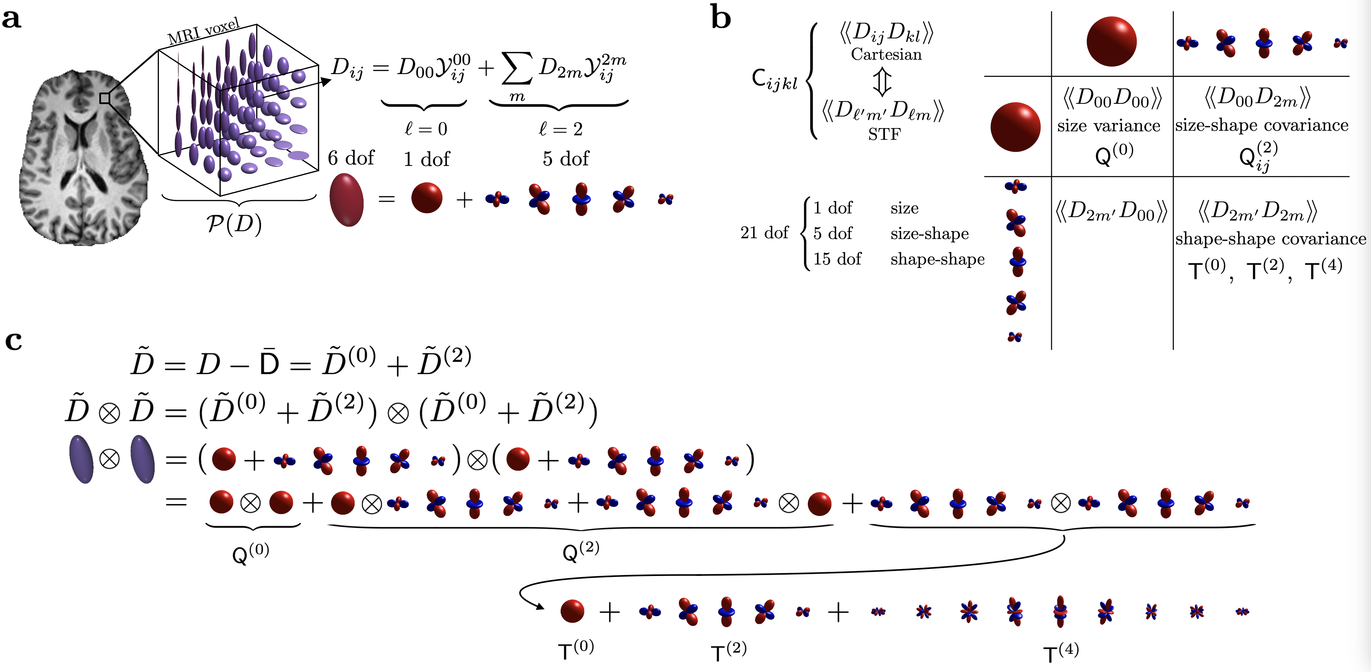
Consider a distribution $$$\mathcal{P}(D)$$$ of Gaussian compartment tensors, Fig.1a. For such tissue:
$$\begin{aligned}\mathsf{D}_{ij}&=\left\langle\,D_{ij}\right\rangle=\sum_\alpha\,f_\alpha\,D_{ij}^\alpha\\\mathsf{C}_{ijkl}&=\left\langle\!\left\langle\,D_{ij}D_{kl}\right\rangle\!\right\rangle\equiv\left\langle\left(D_{ij}-\left\langle\,D_{ij}\right\rangle\right)\left(D_{kl}-\left\langle\,D_{kl}\right\rangle\right)\right\rangle\end{aligned}\quad(3)$$
are the 1st and 2nd central moments of $$$\mathcal{P}(D)$$$ (brackets $$$\langle...\rangle$$$ denote averages over the diffusion tensor distribution while double brackets $$$\langle\langle...\rangle\rangle$$$ denote cumulants).

Similar to Eq.(1), each compartment’s $$$D_{ij}$$$ can be split into irreducible components with $$$\ell=0\,\text{and}\,\ell=2$$$. This is equivalent to superposition of quantum angular momenta $$$\ell=0\,\text{and}\,\ell=2$$$:
$$|D\rangle=D_{00}|0,0\rangle+\sum_mD_{2m}|2,m\rangle.\quad(4)$$
The overall $$$\mathsf{D}$$$ tensor is a mean of these states over $$$\mathcal{P}(D)$$$.

Using Eq.(3), and shifting $$$\tilde{D}=D-\langle\,D\rangle$$$, we symbolically write the angular-momentum representation of the $$$\mathsf{C}$$$-tensor as
$$|\mathsf{C}\rangle=\int\,dD\,\mathcal{P}(D)\,|\tilde{D}\rangle\otimes|\tilde{D}\rangle=\langle\!\langle{D}_{00}D_{00}\rangle\!\rangle\,|0,0\rangle+\sum_m\langle\!\langle{D}_{00}D_{2m}\rangle\!\rangle\,|2,m\rangle+\sum_{m,m’}\langle\!\langle{D}_{2m}D_{2m’}\rangle\!\rangle\,|2,m\rangle\otimes|2,m'\rangle.\quad(5)$$
In other words, the $$$\mathsf{C}$$$-tensor, given by distribution-averaged direct product of states of the form (4), formally maps onto addition of two “superposition states” with “angular momenta” $$$\ell=0$$$ and $$$\ell=2$$$. The object $$$|\mathsf{C}\rangle$$$ is reducible, and splits into irreducible components (Fig.1b,c):
$$\begin{aligned}&\mathrm{Q}^{(0)}\sim\langle\!\langle{D}_{00}D_{00}\rangle\!\rangle\quad\text{(size-size}\,\text{variance)}\\&\mathrm{Q}^{(2)}_M\sim\langle\!\langle{D}_{00}D_{2M}\rangle\!\rangle\quad\text{(size-shape}\,\text{covariance)}\\&\mathrm{T}^{(L)}_M\sim\sum_{m,m'}\langle\!\langle{D}_{2m}D_{2m'}\rangle\!\rangle\,\langle{LM}|2m2m'\rangle,\quad\,L=0,2,4\quad\text{(shape-shape}\,\text{covariance)}\\\end{aligned}\quad(6)$$
given by the corresponding Clebsch-Gordan coefficients⁵ of the addition of angular momenta 2 and 2, obeying the selection rule $$$M=m+m′$$$.
As a result, the space of covariance tensors $$$\mathsf{C}$$$ decomposes into a direct sum of 5 irreducible representations with different $$$\ell=0,2,4$$$:
$$\mathsf{C}\in0\oplus2\oplus0\oplus2\oplus4.\quad(7)$$

Relation to dMRI measurements

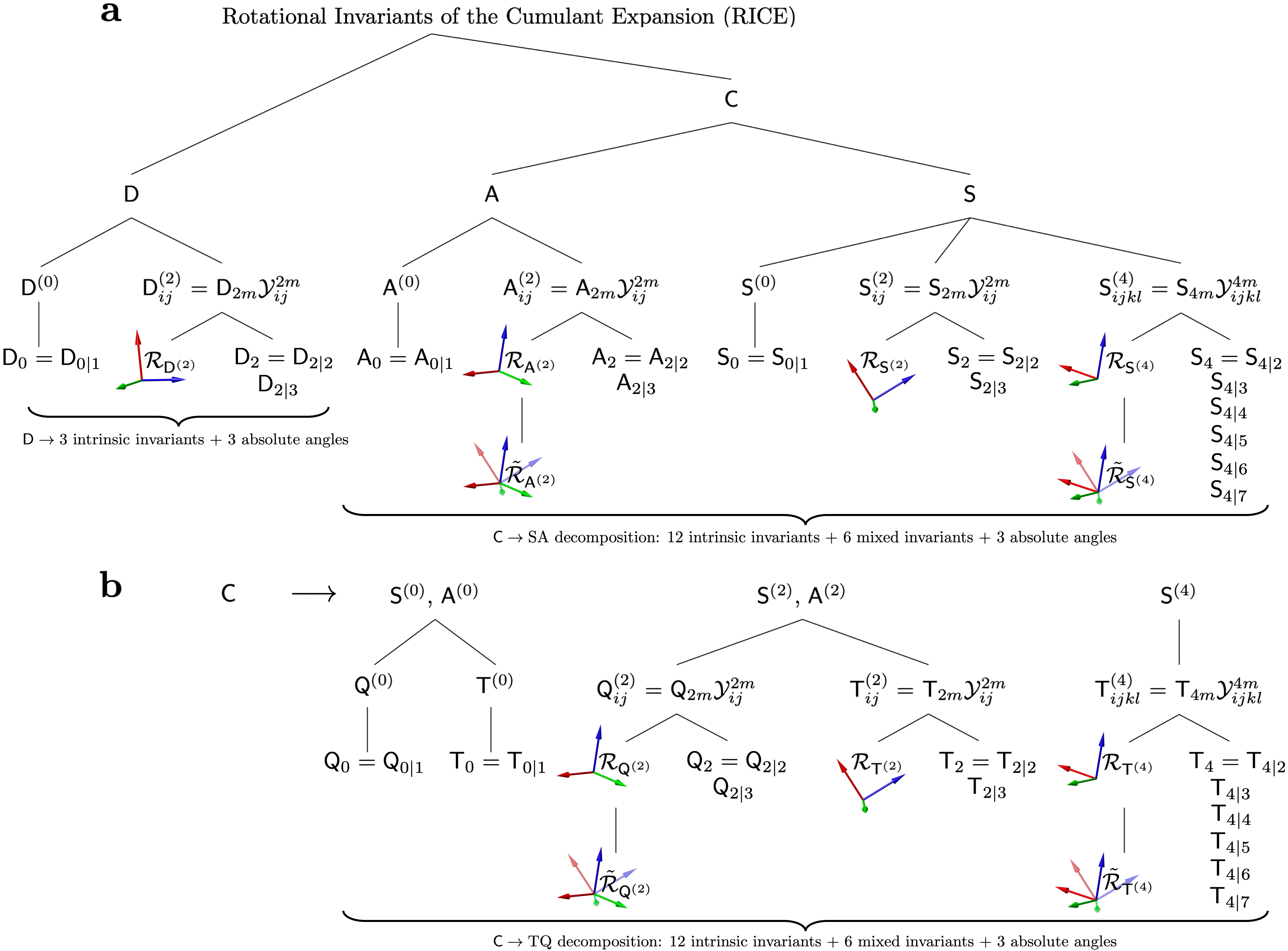
How to proceed from $$$\mathsf{C}_{ijkl}$$$ (Eq.(2)) to $$$\mathsf{T}\,\text{and}\,\mathsf{Q}$$$ and irreducible components? First, we isolate the kurtosis tensor $$$\mathsf{W}_{ijkl}=\frac{3}{\overline{D}^2}\mathsf{S}_{ijkl},\quad\mathsf{S}_{ijkl}=\mathsf{C}_{(ijkl)}$$$, as a fully-symmetric part of $$$\mathsf{C}$$$, having $$$15=1+5+9$$$ dof. It decomposes into irreducible components with $$$\ell=0,2,4$$$ (with dimensions $$$2\ell+1$$$); the asymmetric complement $$$\mathsf{A}=\mathsf{C}-\mathsf{S}$$$ has $$$6=21-15=1+5$$$ degrees of freedom, decomposing into $$$\ell=0,2$$$ components (Fig.3):
$$\begin{aligned}&\mathsf{C}=\mathsf{S}+\mathsf{A}\\&\mathsf{S}=\mathsf{S}^{(0)}+\mathsf{S}^{(2)}+\mathsf{S}^{(4)}\\&\mathsf{A}=\mathsf{A}^{(0)}+\mathsf{A}^{(2)}\end{aligned},\quad(8)$$
One of our main results is the relation between the above $$$\mathsf{S},\,\mathsf{A}$$$ tensors, readily determined from measurements, to the above $$$\mathsf{T},\,\mathsf{Q}$$$ components related to tissue properties:
$$\begin{aligned}&\mathsf{Q}^{(0)}=\frac{5}{9}\mathsf{~S}^{(0)}+\frac{2}{9}\mathsf{~A}^{(0)},\\&\mathsf{Q}^{(2)}=\frac{7}{9}\mathsf{~S}^{(2)}-\frac{2}{9}\mathsf{~A}^{(2)},\\&\mathsf{T}^{(0)}=\frac{4}{9}\mathsf{~S}^{(0)}-\frac{2}{9}\mathsf{~A}^{(0)},\\&\mathsf{T}^{(2)}=\frac{2}{9}\mathsf{~S}^{(2)}+\frac{2}{9}\mathsf{~A}^{(2)},\\&\mathsf{T}^{(4)}=\mathsf{S}^{(4)}.\end{aligned}\quad(9)$$

Rotational invariants of $$$\mathsf{C}$$$

To construct tensor invariants, we split them into those intrinsic to a given representation, and those mixing representations. We define intrinsic invariants as those belonging to a single irreducible component, e.g. $$$\mathsf{S}^{(\ell)},\,\mathsf{T}^{(\ell)}$$$. Conversely, mixed invariants define relative orientations between different irreducible components with $$$\ell>0$$$.

How many invariants are there? For any tensor, the number of invariants equals its number of parameters minus 3, which define its overall orientation^7,8,9. This yields 1 intrinsic invariant for each $$$\ell=0$$$ component; 2 for each $$$\ell=2$$$; and 6 for $$$\ell=4$$$, totalling 12 intrinsic invariants:
$$\begin{aligned}&\mathsf{Q}_0=\mathsf{Q}^{(0)}=\tfrac{1}{3}\mathrm{tr}\mathsf{Q}=\overline{\mathsf{Q}},\\&\mathsf{Q}_{2\mid{n}}=\left(\tfrac{2}{3}\mathrm{tr}\left(\mathsf{Q}^{(2)}\right)^n\right)^{1/n},\quad{n}=2,3,\\&\mathsf{T}_0=\mathsf{T}^{(0)}=\tfrac{1}{5}\mathrm{tr}\mathsf{T}=\overline{\mathsf{T}},\\&\mathsf{T}_{2\mid{n}}=\left(\tfrac{2}{3}\mathrm{tr}\left(\mathsf{T}^{(2)}\right)^n\right)^{1/n},\quad{n}=2,3,\\&\mathsf{~T}_{4\mid{n}}=\left(\tfrac{8}{35}\mathrm{tr}\left(\mathsf{T}^{(4)}\right)^n\right)^{1/n},\quad{n}=2\ldots5,\\&\mathsf{T}_{4\mid{6}}=\mathrm{tr}^{1/3}\mathsf{E}^3,\quad\mathsf{~T}_{4\mid7}=\mathrm{tr}^{1/3}\tilde{\mathsf{E}}^3,\quad\mathsf{E}_{ij}=\sum_a\lambda_a\mathsf{E}_{ij}^{(a)},\quad\text{and}\quad\tilde{\mathsf{E}}_{ij}=\sum_{a\neq{a}_0}\mathsf{E}_{ij}^{(a)},\end{aligned}\quad(10)$$

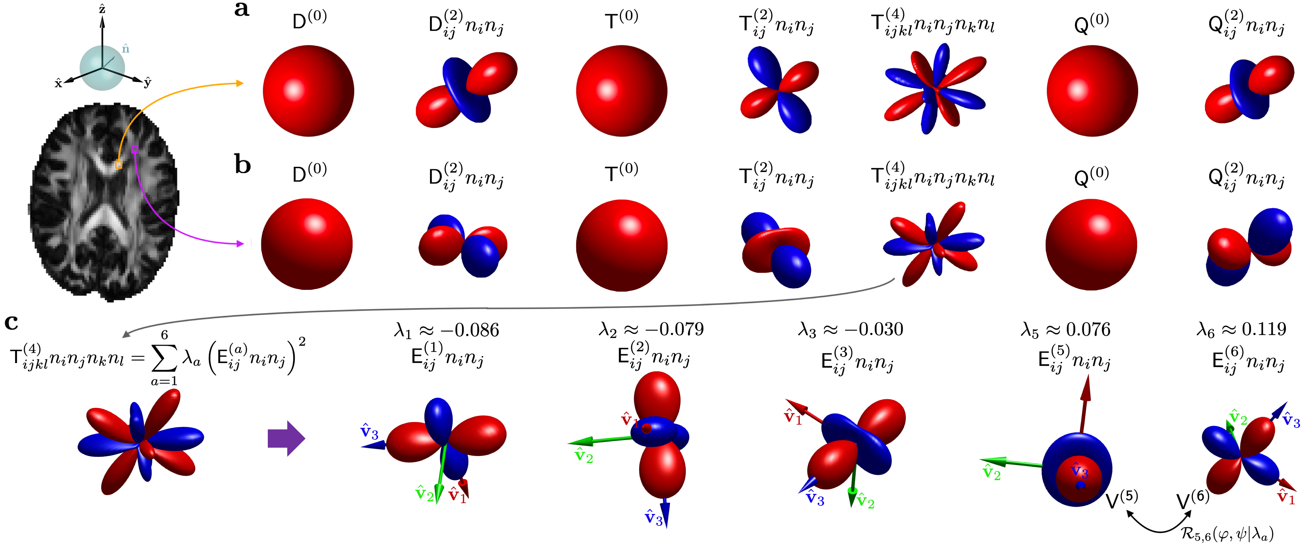
where $$$\mathsf{E}_{ij}^{(a)}$$$ are $$$\mathsf{T}^{(4)}$$$ eigentensors¹⁰.

Given that $$$\mathsf{C}$$$ has $$$21-3=18$$$ total invariants, the remaining $$$6=3+3$$$ are mixed, and can be defined via relative Euler angles between $$$\mathsf{T}^{(2)}-\mathsf{T}^{(4)}$$$ and $$$\mathsf{T}^{(2)}-\mathsf{Q}^{(2)}$$$ eigenframes, Fig.3.

Note that only 7 intrinsic invariants from Eq.(10) suffice to generate all previous model-independent contrasts^1-5 up to $$$b^2$$$ without assumptions on $$$\mathcal{P}(D)$$$:
$$\begin{aligned}\mathrm{MD}&=\mathsf{D}_0,\\\mathrm{FA}&=\sqrt{\tfrac{3\mathsf{D}_2^2}{4\mathsf{D}_0^2+2\mathsf{D}_2{}^2},}\\\mathrm{MK}&=\tfrac{3\mathsf{S}_0}{\mathsf{D}_0^2},\\\mu\mathrm{FA}&=\sqrt{\tfrac{15\mathsf{T}_0+3\mathsf{D}_2^2}{10\mathsf{T}_0+2\mathsf{D}_2^2+12\mathsf{D}_0^2}},\\\mathsf{D}_{\|}^{\text{ax,sym}}&=\mathsf{D}_0+\mathsf{D}_2,\\\mathsf{D}_{\perp}^{\text{ax,sym}}&=\mathsf{D}_0-\tfrac{1}{2}\mathsf{D}_2,\\\mathsf{W}_{\|}^{\text{ax,sym}}&=\mathsf{W}_0+\mathsf{W}_2+\mathsf{W}_4,\\\mathsf{W}_{\perp}^{\text{ax,sym}}&=\mathsf{W}_0-\tfrac{1}{2}\mathsf{~W}_2+\tfrac{3}{8}\mathsf{W}_4,\\\mathbb{V}_{\mathrm{I}}&=\mathsf{Q}_0,\\\mathbb{V}_{\mathrm{A}}&=\mathsf{T}_0+\tfrac{1}{5}\mathsf{D}_2{}^2.\end{aligned}\quad(11)$$

Human Diffusion MRI

A 33-year-old male volunteer underwent MRI in a whole-body 3T-system (Siemens Prisma) using a 20-channel head coil. Maxwell-compensated free-gradient diffusion waveforms yielded linear (30b=1ms/μm2+60b=2ms/μm2) and planar (60b=1.5ms/μm2) b-tensor encoding using a prototype spin echo sequence with EPI readout¹¹. Imaging parameters: voxel-size=2x2x2mm³,TR=4.2s,TE=90ms,bandwidth=1818Hz/Px,Rgrappa=2,pF=6/8,multiband=2. Scan time: 11.5min.

Results and Discussion

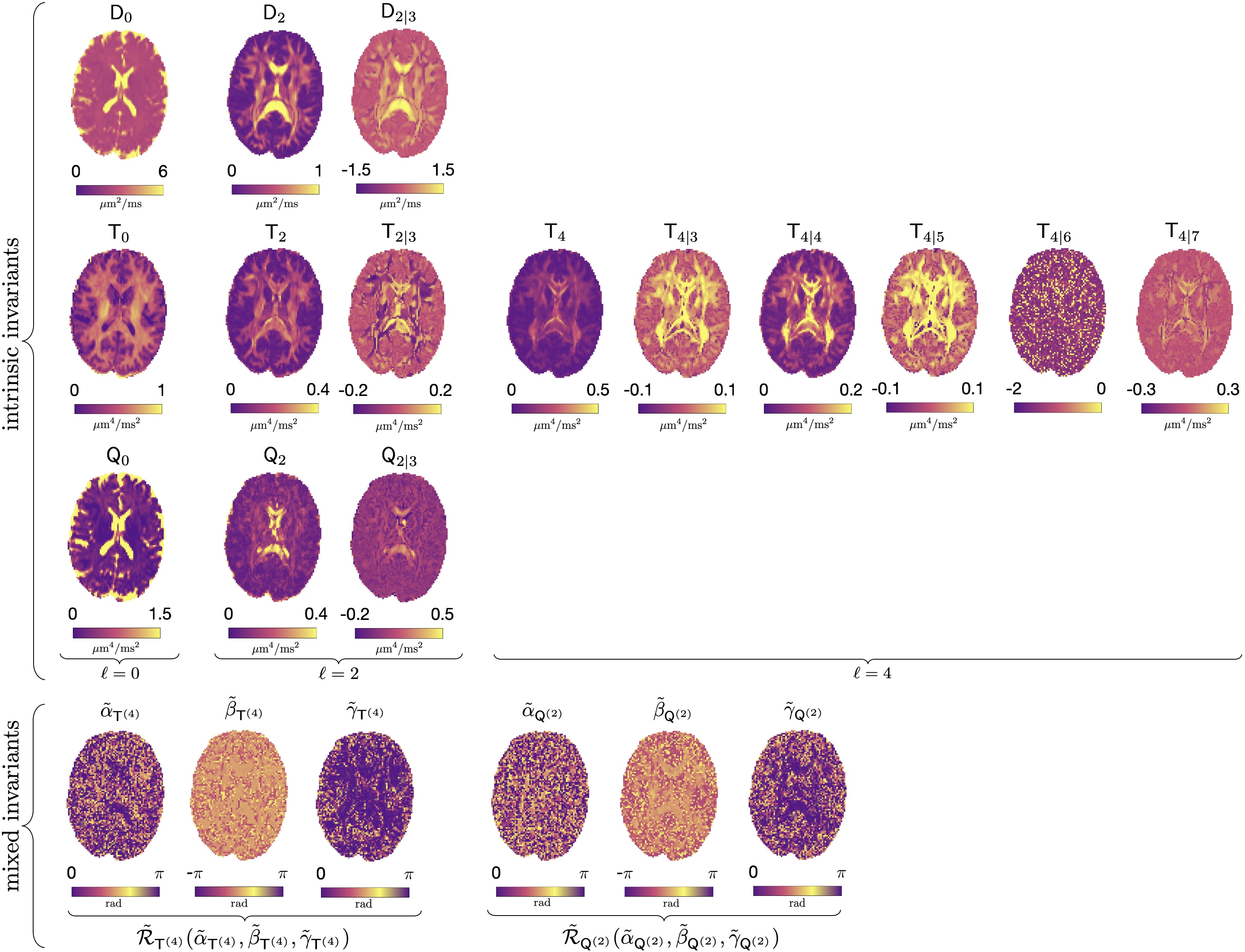
We propose two equivalent irreducible decompositions for $$$\mathsf{C}$$$ with distinct physical meanings: TQ, Eq.(6), splits different sources of compartmental variance ($$$\mathsf{Q}^{(0)},\,\mathsf{Q}^{(2)},\,\mathsf{T}$$$) while SA, Eq.(8), highlights information accessible with LTE ($$$\mathsf{S}$$$) and non-LTE ($$$\mathsf{A}$$$) diffusion-weightings.

Furthermore, we provide a systematic way to compute all rotationally invariant information present in the $$$\mathcal{O}(b^2)$$$ dMRI signal, summarized in Fig.3. Figure 4 shows TQ invariants for a healthy volunteer.

Main 7 RICE maps, $$$\mathsf{S}_{\ell|2}\propto\mathrm{tr}^{1/2}(\mathsf{S}^{(\ell)})^2$$$, Eq.(10), are related to conventional contrasts, Eq.(11). The remaining 14 $$$\mathsf{C}$$$ invariants contain unexplored information.

RICE maps belong to distinct irreducible representations of rotations, and thus, represent “orthogonal” contrasts up to $$$\mathcal{O}(b^2)$$$. Representing the dMRI signal via scalar invariant maps with definite symmetries will underpin machine learning classifiers of brain pathology, development, and aging.

Acknowledgements

This work has been supported by NIH under NINDS awards R01 NS088040, NIBIB award R01 EB027075, and was performed under the rubric of the Center for Advanced Imaging Innovation and Research (CAI2R, www.cai2r.net), an NIBIB National Center for Biomedical Imaging and Bioengineering (NIH P41 EB017183). The authors are grateful to Valerij Kiselev and Sune Jespersen for fruitful discussions.

References

1. Basser, P. J., Mattiello, J. & LeBihan, D. Estimation of the Effective Self-Diffusion Tensor from the NMR Spin Echo. J. Magn. Reson. 103, 247–254 (1994).

2. Jensen, J. H., Helpern, J. A., Ramani, A., Lu, H. & Kaczynski, K. Diffusional Kurtosis Imaging: The Quantification of Non-Gaussian Water Diffusion by Means of Magnetic Resonance Imaging. Magn. Reson. Med. 53, 1432–1440 (2005).

3. Westin, C.-F. et al. q-space trajectory imaging for multidimensional diffusion MRI of the human brain. NeuroImage 135, 345–362 (2016).

4. Szczepankiewicz, F. et al. The link between diffusion MRI and tumor heterogeneity: Mapping cell eccentricity and density by diffusional variance decomposition (DIVIDE). NeuroImage 142, 522–532 (2016).

5. Coelho, S., Fieremans, E. & Novikov, D. S. Rotational invariants of the cumulant expansion (RICE). in Proceedings of the International Society of Magnetic Resonance in Medicine vol. 0751 (Wiley, 2022).

6. Tinkham, M. Group Theory and Quantum Mechanics (Dover Books on Chemistry). (Dover Publications, 2003).

7. Betten, J. Invariants of fourth-order tensors. in Applications of tensor functions in solid mechanics (ed. Boehler, J.-P.) 203–226 (Springer-Verlag, 1987).

8. Ghosh, A., Papadopoulo, T. & Deriche, R. Biomarkers for HARDI: 2nd & 4th order tensor invariants. in 2012 9th IEEE International Symposium on Biomedical Imaging (ISBI) 26–29 (2012).

9. Papadopoulo, T., Ghosh, A. & Deriche, R. Complete Set of Invariants of a 4thOrder Tensor: The 12 Tasks of HARDI from Ternary Quartics. in Medical Image Computing and Computer-Assisted Intervention – MICCAI 2014 233–240 (Springer International Publishing, 2014).

10. Basser, P. J. & Pajevic, S. Spectral decomposition of a 4th-order covariance tensor: Applications to diffusion tensor MRI. Signal Process. 87, 220–236 (2007).

11. Szczepankiewicz, F., Westin, C.-F. & Nilsson, M. Maxwell-compensated design of asymmetric gradient waveforms for tensor-valued diffusion encoding. Magn. Reson. Med. 82, 1424–1437 (2019).

Figures

Figure 1. a) An MRI voxel as a distribution of compartment diffusion tensors $$$D$$$ decomposed in STF/SH basis. b) Irreducible components of the TQ decomposition represent 1 size-size, 5 size-shape, and 1 + 5 + 9 shape-shape covariances in the 21 dof of C. c) TQ decomposition is tissue-driven. Central moments of compartment tensors $$$D$$$ correspond to tensor products that map onto the addition of angular momenta, Eq.(5), subsequently averaged over $$$\mathcal{P}(D)$$$.

Figure 2. TQ decomposition of D and C, Eqs.(1-6), for 2 WM voxels: (a) corpus callosum - aligned fibers, and (b) longitudinal superior fasciculus - crossing fibers. Glyphs are rescaled and color-coded by their signs, their radius represents the absolute value. (c) Eigentensor decomposition¹⁰ of $$$\mathsf{T}^{(4)}$$$ for the voxel in (b). The 6 invariants of $$$\mathsf{T}_{ijkl}^{(4)} = \mathsf{S}_{ijkl}^{(4)}$$$ correspond to 4 degrees of freedom from $$$\lambda_a$$$ and 2 dof defining the relative orientations among any pair of eigentensors $$$\mathsf{E}_{ij}^{(a)}$$$.

Figure 3. Irreducible decompositions of D and C and their invariants: a) SA decomposition, Eq.(8). b) TQ decomposition, Eq.(6). Each irreducible component has its intrinsic invariants (1 for $$$\ell=0$$$; 2 for $$$\ell=2$$$; and 6 for $$$\ell=4$$$). Together with these 1+2+1+2+6=12 intrinsic invariants, C has 3 · 3 = 9 basis-dependent absolute angles defining the orientations of its $$$S^{(2)},\,S^{(4)},\,A^{(2)}$$$ components via their rotation matrices, such that total dof count of C is 21 = 12 + 9. Out of 9 dof defining the three rotation matrices, 6 are mixed invariants.

Figure 4. RICE maps for a normal brain (33 y.o. male). Intrinsic invariants for each irreducible decomposition of $$$\mathsf{D},\,\mathsf{T},\,\mathsf{Q}$$$ are shown as powers of corresponding traces, to match units of $$$\mathsf{D}$$$ and $$$\mathsf{C}$$$. Only 7 intrinsic invariants generate all previously studied model-independent O(b²) dMRI contrasts, Eq.(11). The 6 mixed invariants represent relative angles between eigenframes of $$$T^{(4)},\,Q^{(2)}$$$, and $$$T^{(2)}$$$. The underlying tissue microstructure introduces correlations between invariants.

Proc. Intl. Soc. Mag. Reson. Med. 32 (2024)

0641

DOI: https://doi.org/10.58530/2024/0641