0544
PhyCHarm : Physics-Constrained Deep Neural Networks for Multi-Scanner Harmonization1Biomedical Engineering, Hankuk University of Foreign Studies, Yongin-si, Korea, Republic of, 2Computer Science, Georgia State University, Atlanta, GA, United States
Synopsis
Keywords: Analysis/Processing, Machine Learning/Artificial Intelligence, Data Harmonization, Bloch equation
Motivation: The MR scanner effect in a multi-site dataset can affect bias in statistical analysis or reduce generality in deep neural networks.
Goal(s): We aim to suggest a MR physics-informed harmonization framework (PhyCHarm) that generates consistent quantitative maps and harmonized T1w images.
Approach: We introduce a Quantitative Maps Generator and a Harmonization Network to be trained with a constraint loss based on a signal equation.
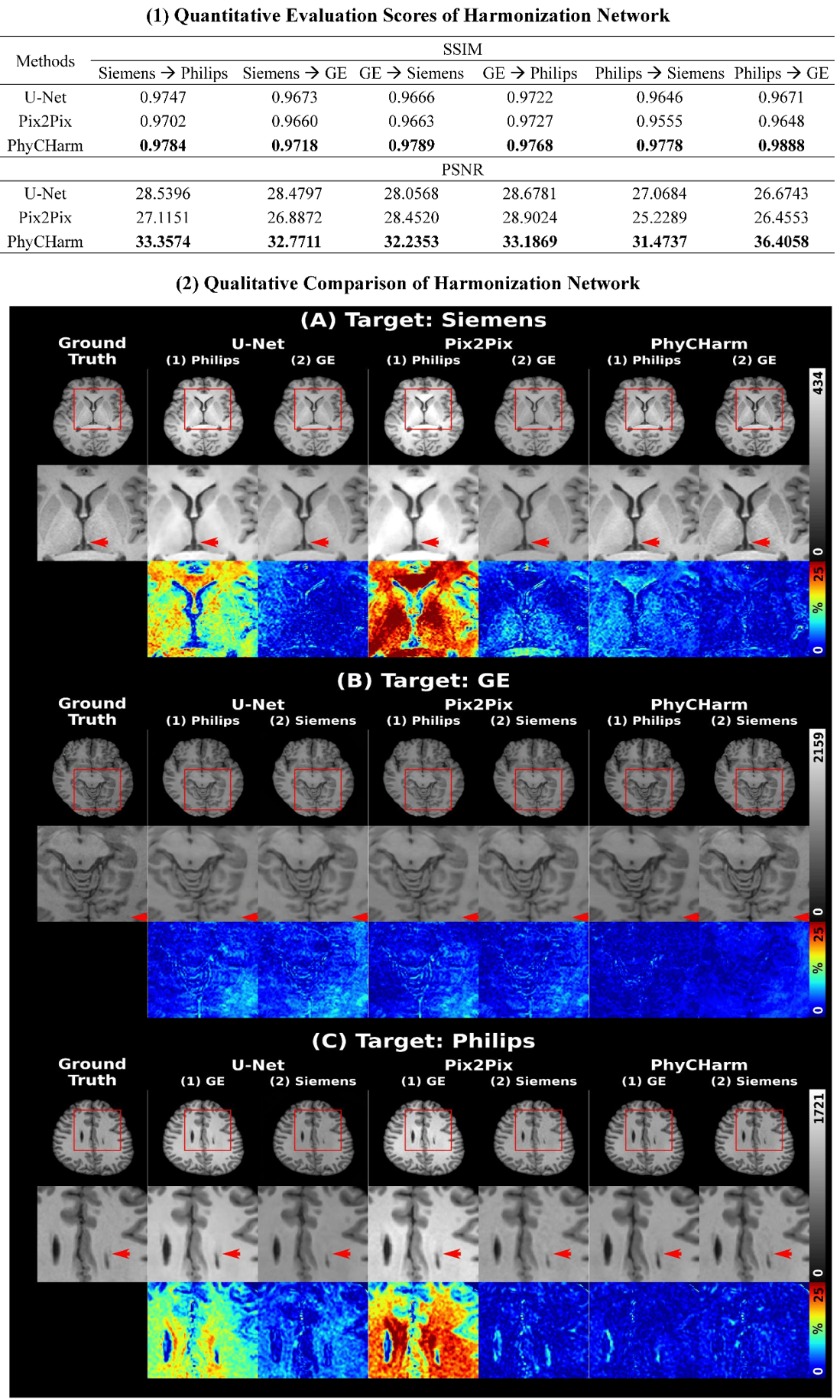
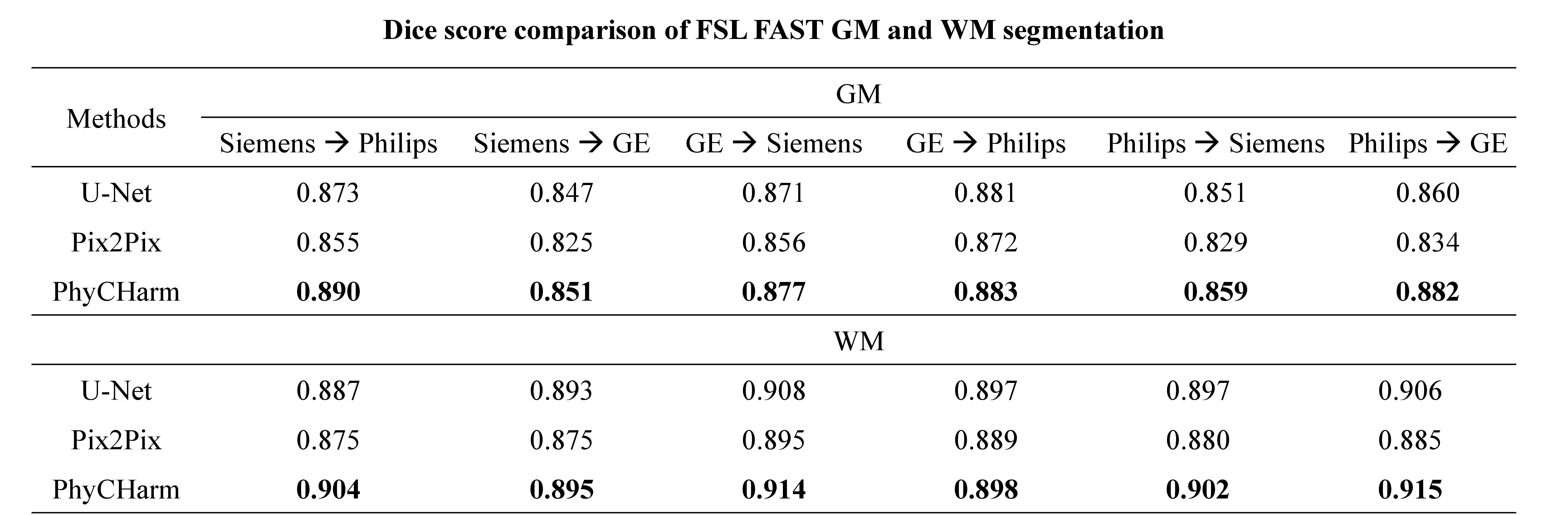
Results: PhyCHarm shows the highest evaluation scores in both networks and consistent segmentation accuracy in the downstream task (FSL FAST GM and WM segmentation).
Impact: PhyCHarm works based on the Bloch equation. PhyCHarm enables us to reduce scanner effects efficiently in the dataset before conducting test/retest, longitudinal, or multi-site studies. It can be helpful to ensure deep neural networks' generality.
Introduction
Variations in the MR scanner, such as differences in gradient conditions, coil sensitivity, and the optimal values of each scan parameter, can impact MRI signals. These variations can introduce bias in results when dealing with large multi-site MRI datasets for statistical analysis or deep neural network training. To address this, harmonization methods have been suggested with the united acquisition tool or deep learning-based methods1-8. However, generative network-based methods have shown a risk of generating inaccurate anatomical features2,4,6. This study suggests an end-to-end Physics-Constrained deep neural network for multi-site MR Harmonization, PhyCHarm. (PhyCHarm is an improved version of the 2023 ISMRM abstract9). PhyCHarm ensures the high quality of harmonized T1w while reducing motion artifacts in generated quantitative maps by incorporating the Bloch equation as a training constraint.Methods

The PhyCHarm has two networks: (1) Quantitative Maps Generator and (2) Harmonization Network. Figure 1 shows the inference pipeline. The Quantitative Maps Generator generates T1-map and M0-map, and then the Bloch equation is utilized to calculate constrained T1w images. The Harmonization Network works to harmonize T1w images across Siemens, GE, and Philips.Quantitative Maps Generator
1) Dataset
We used an open dataset, MICA-MICs10, consisting of INV1, INV2, T1w, and T1-map acquired from MP2RAGE sequence11. M0-map was generated from INV2 and T1-map through the inversion recovery signal equation. We used 20 subjects for training, 5 for validation, and 25 for inference.
2) Preprocessing
Brain reorientation was conducted to align axial slices along the z-axis using FSL12, FOV crop was carried out using ANTsPy13, and skull stripping was completed using HD-BET14.
3) Training Quantitative Maps Generator
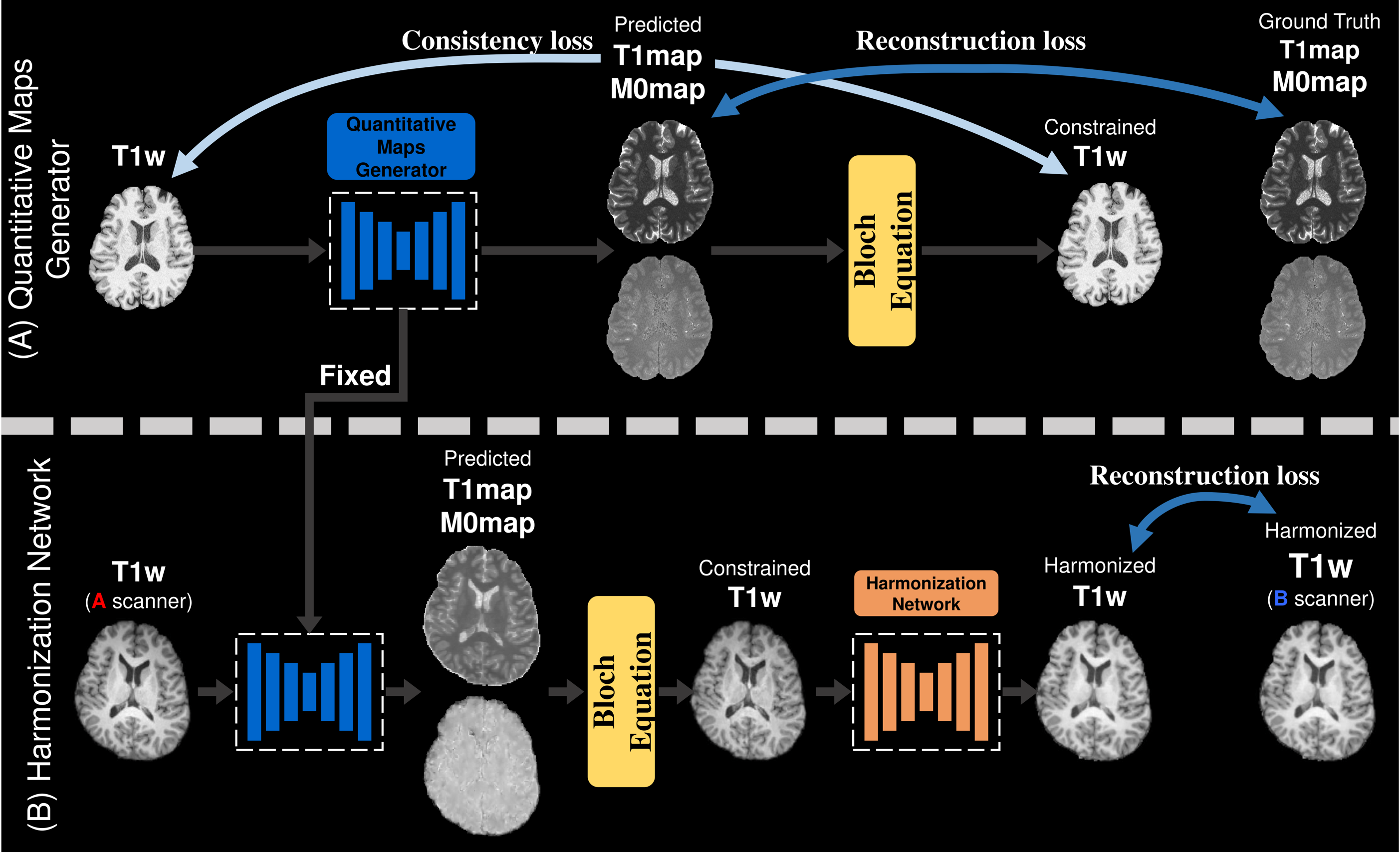
Figure 2(A) illustrates the training pipeline of the Quantitative Maps Generator. The network was trained using 2D-U-Net15, MSE loss, and the ADAM16 optimizer with a learning rate 0.001. The total loss ($$$\mathcal{L}_{total}$$$) is defined as a weighted sum of the reconstruction loss ($$$\mathcal{L}_{T_{1}}$$$, $$$\mathcal{L}_{M_{0}}$$$) and the consistency loss ($$$\mathcal{L}_{cons}$$$).
$$\mathcal{L}_{total} = \lambda_{1}\times\mathcal{L}_{T_{1}} + \lambda_{2}\times\mathcal{L}_{M_{0}}+\lambda_{3}\times{L}_{cons}$$
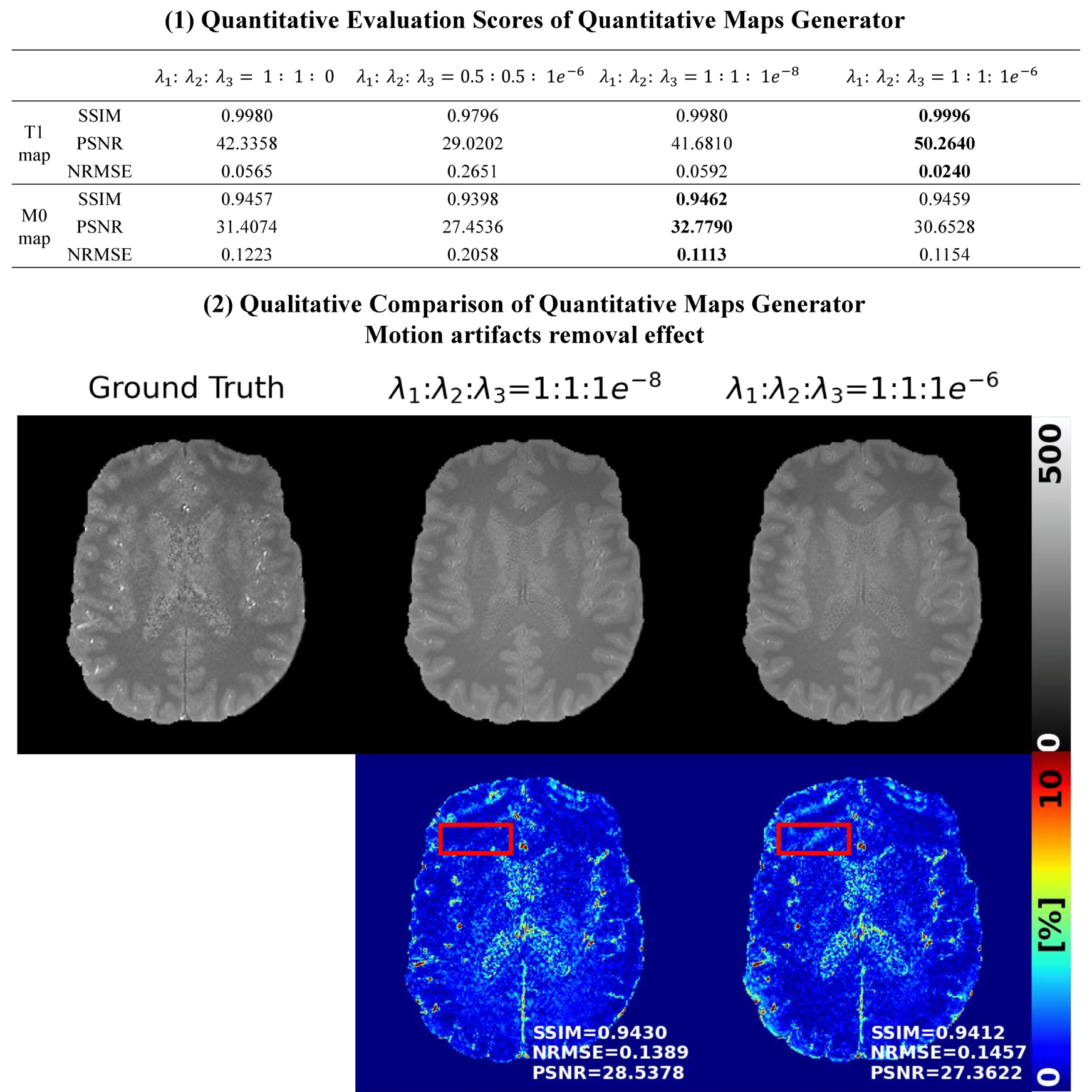
where λ1=1, λ2=1, λ3=1e-6. These values were defined experimentally.
The reconstruction loss was calculated between the predicted maps and the ground truth. The consistency loss was computed between the constrained T1w (ConsT1w) and the input T1w. The ConsT1w is generated as below:
$$T1w = M0 \times (1-2\times exp^{-\frac{TI}{T1}}+exp^{-\frac{TR}{T1}})\times exp^{-\frac{TE}{T2}}$$
$$consT1w' = \hat{M0}\times(1-2\times exp^{-\frac{TI}{\hat{T1}}}+exp^{-\frac{TR}{\hat{T1}}})$$
$$\hat{T2}term =\frac{T1w}{consT1w'}
=exp^{-\frac{TE}{T2}}$$
$$consT1w =\hat{M0}\times(1-2\times exp^{-\frac{TI}{\hat{T1}}}+exp^{-\frac{TR}{\hat{T1}}})\times\hat{T2}term $$
By using the inversion-recovery signal equation for T1w, we generated without the T2 term ($$$exp^{-\frac{TE}{T2}}$$$), employing a predicted M0map ($$$\hat{M0}$$$), a predicted T1map ($$$\hat{T1}$$$), TI / TR = 2830 / 5000 ms. To generate consT1w with $$$\hat{T2}term$$$, we calculated $$$\hat{T2}term$$$ by dividing the input T1w by consT1w'. Then, consT1w is used as a training constraint.
Harmonization Network
1) Dataset
T1w images (IRB-approved) of four healthy traveling subjects from three scanners at different sites were used: Siemens Trio (3T), GE SIGNA (3T), and Philips Ingenia CS (3T).
2) Preprocessing
The preprocessing method used for the Quantitative Maps Generator was utilized for the Harmonization Network dataset. To standardize the voxel size to 0.8 iso-voxel, we applied resampling to the GE dataset using spline interpolation. Subsequently, an affine registration was utilized to align the spatial orientation of the Siemens and Philips datasets to match that of the GE dataset. Finally, N4 bias correction17 was applied.
3) Training Harmonization Network
Figure 2(B) displays the training pipeline of the Harmonization Network. It was trained to generate a harmonized T1w image from the constrained T1w image for each pair of the traveling dataset: (a) GE and Siemens, (b) Siemens and Philips, and (c) Philips and GE. The pre-trained Quantitative Maps Generator was utilized to generate T1-map and M0-map of each source scanner’s T1w images while its parameters were all fixed. The ConsT1w was generated using the following equations:
$$consT1w_{source}'= \hat{M0}_{source}\times(1-2\times exp^{-\frac{TI_{source}}{\hat{T1}_{source}}}+exp^{-\frac{TR_{source}}{\hat{T1}_{source}}})$$
$$\hat{T2}term=\frac{T1w_{source}}{consT1w_{source}'} = exp^{-\frac{TE}{T2}}$$
$$\hat{T2} = -\frac{TE_{source}}{\log{\hat{T2}term}}$$
$$consT1w_{target} = \hat{M0}_{source}\times(1-2\times exp^{-\frac{TI_{target}}{\hat{T1_{source}}}}+exp^{-\frac{TR_{target}}{\hat{T1}_{source}}})\times exp^{-\frac{TE_{target}}{\hat{T2}}}$$
where consT1wtarget is the input of the Harmonization Network.
The Harmonization Network was trained using 2D U-Net, the reconstruction loss based on the MSE loss, and the ADAM optimizer with a learning rate of 0.001. To avoid over-fitting, we applied 4-fold cross-validation and dropout with 0.1 of the probability.
Results
Figure 3 shows the evaluation scores and the impact of motion artifact minimization achieved using the Quantitative Maps Generator. Figure 4 represents the comparison results of PhyCHarm with U-Net and Pix2Pix18. Figure 5 compares segmentation consistency for GM and WM through FSL FAST.Discussion and Conclusion
In this study, we provide evidence that incorporating the Bloch equation during the training of deep neural networks results in improved quality for both harmonized T1w images and quantitative maps, notwithstanding the restricted size of our training dataset.Acknowledgements
This work was supported by the National Research Foundation of Korea (NRF) grant funded by the Korea government (MSIT) (NRF-2023R1A2C1007292)References
1. Dewey BE, Zhao C, Reinhold JC, et al. DeepHarmony: A deep learning approach to contrast harmonization across scanner changes. Magnetic resonance imaging. 2019;64:160-70.2. Zuo L, Dewey BE, Liu Y, et al. Unsupervised MR harmonization by learning disentangled representations using information bottleneck theory. NeuroImage. 2021;243:118569.
3. Moyer D, Ver Steeg G, Tax CM, Thompson PM. Scanner invariant representations for diffusion MRI harmonization. Magnetic resonance in medicine. 2020;84(4):2174-89.
4. Torbati ME, Minhas DS, Laymon CM, et al. MISPEL: A supervised deep learning harmonization method for multi-scanner neuroimaging data. Medical image analysis. 2023;89:102926.
5. Ren M, Dey N, Fishbaugh J, Gerig G. Segmentation-renormalized deep feature modulation for unpaired image harmonization. IEEE transactions on medical imaging. 2021;40(6):1519-30.
6. Guan H, Liu Y, Yang E, et al. Multi-site MRI harmonization via attention-guided deep domain adaptation for brain disorder identification. Medical image analysis. 2021;71:102076.
7. Bashyam VM, Doshi J, Erus G, et al. Deep generative medical image harmonization for improving cross‐site generalization in deep learning predictors. Journal of Magnetic Resonance Imaging. 2022;55(3):908-16.
8. Karakuzu A, Biswas L, Cohen‐Adad J, Stikov N. Vendor‐neutral sequences and fully transparent workflows improve inter‐vendor reproducibility of quantitative MRI. Magnetic Resonance in Medicine. 2022;88(3):1212-28.
9. Lee G, Lee J, Ye D-H, Oh S-H. Bloch-informed neural network for multi-scanner MR Harmonization. International Society for Magnetic Resonance in Medicine, 2023.
10. Royer J, Rodríguez-Cruces R, Tavakol S, et al. An open MRI dataset for multiscale neuroscience. Scientific Data. 2022;9(1):569.
11. Marques JP, Kober T, Krueger G, et al. MP2RAGE, a self bias-field corrected sequence for improved segmentation and T1-mapping at high field. Neuroimage. 2010;49(2):1271-81.
12. Smith SM, Jenkinson M, Woolrich MW, et al. Advances in functional and structural MR image analysis and implementation as FSL. Neuroimage. 2004;23:S208-S19.
13. Tustison NJ, Cook PA, Holbrook AJ, et al. The ANTsX ecosystem for quantitative biological and medical imaging. Scientific reports. 2021;11(1):9068.
14. Schell M, Tursunova I, Fabian I, et al. Automated brain extraction of multi-sequence MRI using artificial neural networks. 2019. European Congress of Radiology-ECR 2019.
15. Ronneberger O, Fischer P, Brox T. U-net: Convolutional networks for biomedical image segmentation. Medical Image Computing and Computer-Assisted Intervention–MICCAI 2015: 18th International Conference, Munich, Germany, October 5-9, 2015, Proceedings, Part III 18, 2015. Springer: 234-41.
16. Kingma DP, Ba J. Adam: A method for stochastic optimization. arXiv preprint arXiv:1412.6980. 2014.
17. Tustison NJ, Avants BB, Cook PA, et al. N4ITK: improved N3 bias correction. IEEE transactions on medical imaging. 2010;29(6):1310-20.
18. Isola P, Zhu J-Y, Zhou T, Efros AA. Image-to-image translation with conditional adversarial networks. Proceedings of the IEEE conference on computer vision and pattern recognition, 2017. 1125-34.
Figures