0528
Non-idealized system (NIS) optimization of EPI sequences at ultra-high field.1Biomedical Engineering Department, King's College London, London, United Kingdom, 2Max Planck Institute for Biological Cybernetics, University of Tübingen, Tübingen, Germany, 3Institute of Neuroradiology, Universitätsklinik Erlangen, Erlangen, Germany, 4MR Research Collaborations, Siemens Healthcare Limited, Frimley, United Kingdom, 5Department of Artificial Intelligence in Biomedical Engineering, Friedrich-Alexander-Universität Erlangen-Nürnberg, Erlangen, Germany, 6Centre for the Developing Brain, King's College London, London, United Kingdom
Synopsis
Keywords: System Imperfections, Pulse Sequence Design
Motivation: MRI scanners are built under the assumption of near perfect responses of each subsystem. Computing advances mean that this may no longer be necessary, enabling exploration of cheaper, efficient alternatives.
Goal(s): To allow high-performance scanning with less emphasis on hardware performance, reducing costs and improving access.
Approach: We consider non-idealized system optimization where hardware imperfections are built into a forward model used to optimize pulse sequences via the MR-zero framework. We experimentally demonstrate NIS using measured GIRFs from a 7T system to optimize EPI sequences.
Results: NIS optimization produces sequences that substantially reduce image artefacts even for scenarios that previously exceeded hardware constraints.
Impact: NIS optimization embraces gradient system imperfections, discovering novel acquisition strategies to inherently mitigate them. Although demonstrated on a state-of-the-art 7T scanner, the concept of including imperfections directly into sequence design offers a means to maximize performance of any scanner hardware.
Introduction
MRI scanners are typically built using an 'idealized independent subsystem' design philosophy in which each hardware subsystem is engineered to produce near-perfect responses so that they can be considered ideal from the perspective of sequence design. Computing advances mean that this paradigm may no longer be required, enabling exploration of more efficient or cheaper alternatives.Recently we proposed non-idealized system (NIS) optimization that accounts for system imperfections and learns strategies to overcome them, demonstrating its theoretical performance to counter eddy currents (1). The framework draws a distinction between demanded waveforms $$$g(t)$$$ and realized waveforms $$$G(t)$$$. The method optimizes $$$g(t)$$$ subject to hardware limits and an image loss function calculated by simulating performance based on predicted $$$G(t)$$$ (Figure 1B). Previously $$$g(t)$$$ was related to $$$G(t)$$$ via a simple exponential eddy current model; here we generalize to an empirically measured 'gradient impulse response function' (GIRF) $$$h(t)$$$ that directly characterizes actual gradient performance, including cross-terms between gradient axes (2).
Methods
Experiments were conducted on a 7T scanner (MAGNETOM Terra, Siemens Healthcare, Erlangen, Germany). GIRF measurement was made using an image-based method with a spherical water phantom and variable amplitude chirp test waveform (3). The forward model includes 'cross-terms' between gradients:$$[1]\;\bf{G=h*g}$$
$$[2]\;\left[\begin{array}{c}G_x(t)\\G_y(t)\\G_z(t)\\\end{array}\right]=\left[\begin{array}{ccc}h_{xx}(t)&h_{yx}(t)&h_{zx}(t)\\h_{xy}(t)&h_{yy}(t)&h_{zy}(t)\\h_{xz}(t)&h_{yz}(t)&h_{zz}(t)\\\end{array}\right]*\left[ \begin{array}{c}g_x(t)\\g_y(t)\\g_z(t)\\\end{array}\right]$$
implemented as a time-domain convolution; see Figure 2 for $$$h(t)$$$ examples. We considered EPI sequences (Figure 3) with inter-echo spacing 0.73-2.61ms and fixed single ADC duration of 0.63ms (0.1-0.3s scan times). Adam optimization (4) minimized error between an ideal target and predicted images reconstructed using a simple inverse Fourier transform (iFFT) assuming original k-space sample locations.
The free parameters are demanded amplitudes at the raster time points defining $$$g(t)$$$, which are optimized subject to slew rate and amplitude constraints (180mT/m/ms; 72mT/m), with the forward model (including the GIRF) used to simulate k-space data. The optimization utilizes the end-to-end MR-zero framework (5) based on phase distribution graph simulation (6).
All target sequences had FOV=250mm with matrix size 64x64; optimized sequences were implemented on the scanner using pulseq (7) and tested on both a spherical water phantom and healthy volunteer (male, age 28). Presented images were reconstructed offline using iFFT on acquired k-space data with no corrections.
Results
Figure 4A illustrates simulated images for a numerical brain phantom showing the target image (forward model assuming ideal scanner performance); the forward model including the GIRF showing considerable Nyquist ghosting in all cases; and the result after optimization with ghosting absent. Figure 4B shows images obtained using the same sequences on a spherical water phantom. Optimized sequences consistently show much reduced ghosting, as per simulated predictions. For the shortest echo spacing (0.73ms), NIS optimization yields a sequence that generates ghost-free images, whereas the initial version cannot run as it violates slew rate limits.Figure 5A shows results from a sequence with echo spacing 0.81ms on a volunteer; as for phantom scans, the initial sequence has ghosting that is resolved by the optimal sequence. Figure 4 shows initial and optimized gradient inputs $$$g(t)$$$ and predicted fields $$$G(t)$$$ as well as predicted k-space sample locations (from integrating $$$G(t)$$$). The unoptimized sequence does not hit the correct sample locations (integer increments on this plot) whereas the optimized one does. Figure 5B shows results for an example optimized sequence that cannot be realized without violating slew rate constraints using standard sequence design.
Discussion and Conclusions
NIS optimization was extended to include empirically measured GIRF and resolves image imperfections in EPI data at 7T. The GIRF included all pre-emphasis steps implemented by the scanner manufacturer, so our results represent real-world performance improvement. NIS optimization essentially pre-distorts the readout gradient to compensate for low-pass behavior. We use a simple iFFT image reconstruction, thereby forcing data to match this. An alternative retrospective correction method would employ the GIRF to predict k-space trajectories used for reconstruction (8). NIS optimization improves data quality and could ultimately be used with less optimal hardware or paired with a reconstruction approach to further improve performance. Even neural network reconstruction or post-processing can be trained simultaneously in the end-to-end learning (9,10).The example of EPI on a 7T system illustrates how knowledge of system performance could be used to obtain high-quality data from non-ideal hardware. This concept generalizes to any scanner and we envisage that the system model could be extended to include any system imperfection. For example, Albert et al. (11) characterized RF power amplifier performance in a low-cost, low-field setting using an empirically trained neural network model. Examples presented here used a coarse imaging resolution to limit computational times to ~1hr per optimization; future work aims to accelerate these predictions.
Acknowledgements
The research was supported by core funding from the Wellcome/EPSRC Centre for Medical Engineering [WT203148/Z/16/Z] and by the National Institute for Health Research (NIHR) Biomedical Research Centre based at Guy's and St Thomas' NHS Foundation Trust and King's College London and/or the NIHR Clinical Research Facility. The views expressed are those of the author(s) and not necessarily those of the NHS, the NIHR or the Department of Health and Social Care.References
1. West DJ, Glang F, Endres J, Zaiss M, Malik SJ, Hajnal J V. Overcoming system imperfections using end-to-end MR sequence design. In: Proc. Intl. Soc. Mag. Reson. Med. 31. (2023)
2. Addy NO, Wu HH, Nishimura DG. Simple method for MR gradient system characterization and k-space trajectory estimation. Magn. Reson. Med. 2012;68:120–129 doi: 10.1002/mrm.23217.
3. West DJ, Leitão D, Tomi-Tricot R, Wood TC, Hajnal J V., Malik SJ. Characterizing gradient performance and estimating Maxwell fields at 0.55T. In: Proc. Intl. Soc. Mag. Reson. Med. 31. (2023)
4. Kingma DP, Ba JL. Adam: a method for stochastic optimization. arXiv 2014;1412.6980:1–15.
5. Loktyushin A, Herz K, Dang N, et al. MRzero - Automated discovery of MRI sequences using supervised learning. Magn. Reson. Med. 2021;86:709–724 doi: 10.1002/mrm.28727.
6. Endres J, Dang N, Glang F, Loktyushin A, Weinmüller S, Zaiss M. Phase distribution graphs for differentiable and efficient simulations of arbitrary MRI sequences. In: Proc. Intl. Soc. Mag. Reson. Med. 30. (2022)
7. Layton KJ, Kroboth S, Jia F, et al. Pulseq: A rapid and hardware-independent pulse sequence prototyping framework. Magn. Reson. Med. 2017;77:1544–1552 doi: https://doi.org/10.1002/mrm.26235.
8. Vannesjo SJ, Graedel NN, Kasper L, et al. Image reconstruction using a gradient impulse response model for trajectory prediction. Magn. Reson. Med. 2016;76:45–58 doi: 10.1002/mrm.25841.
9. Dang HN, Endres J, Weinmüller S, et al. MR-zero meets RARE MRI: Joint optimization of refocusing flip angles and neural networks to minimize T2-induced blurring in spin echo sequences. Magn. Reson. Med. 2023;90:1345–1362 doi: 10.1002/mrm.29710.
10. Dang HN, Endres J, Weinmüller S, Maier A, Knoll F, Zaiss M. Simultaneous optimization of MR sequence and reconstruction using MR-zero and variational networks. In: Proc. Intl. Soc. Mag. Reson. Med. 31. (2023)
11. Albert MM, Vaughn CE, Martin JB, Srinivas SA, Grissom WA. RF Pulse Predistortion for Low-Field MRI Based on Spin Physics Using a Neural Network Amplifier-to-Bloch Equation Model. In: Proc. Intl. Soc. Mag. Reson. Med. 31. (2023)
Figures
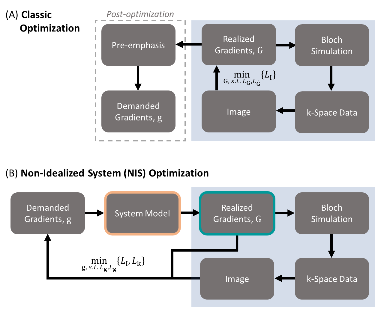
Figure 1: Gradient design strategies. (A) Classic approach optimizes $$$G(t)$$$ assuming ideal performance with optional pre‑calibrated correction applied to $$$g(t)$$$ at run-time. (B) NIS optimization optimizes $$$g(t)$$$ by directly predicting $$$G(t)$$$ using a comprehensive forward model (here, including a GIRF). NIS optimization has: an image loss to promote similarity to a target image ($$$L_I$$$); a k-distance loss to promote sampling locations that lie on a Cartesian grid ($$$L_k$$$); and $$$L_g$$$/$$$L_{\dot{g}}$$$ to satisfy amplitude/slew rate constraints.
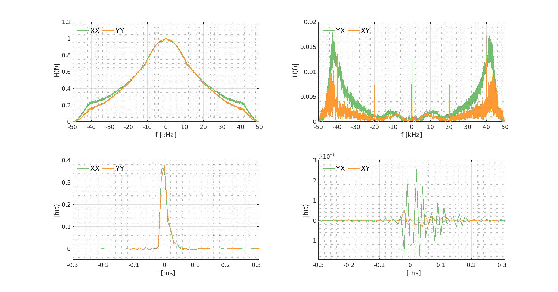
Figure 2: GIRF of the 7T system expressed in the frequency-domain ($$$H(f)$$$) and time-domain ($$$h(t)$$$). The latter are convolved with the demanded gradient waveforms to predict acquired image quality. For the cross-terms (RHS plots), the first character denotes the axis on which a gradient response is measured due to a gradient applied along the axis denoted by the second character. Cross-terms measured along X and Y have a magnitude of less than 1% of the self-terms.
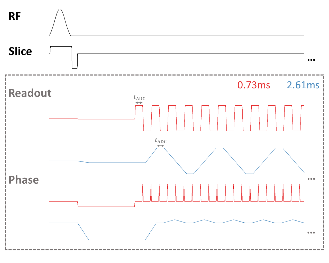
Figure 3: Schematic showing the EPI sequences considered in this work. Seven sequences were optimized and implemented though only those with the shortest and longest echo spacings are plotted here to illustrate the differences between gradient structure. RF and slice-selection gradients remain unchanged, whereas readout and phase-encoding gradients are optimizable (indicated by the dashed gray box).
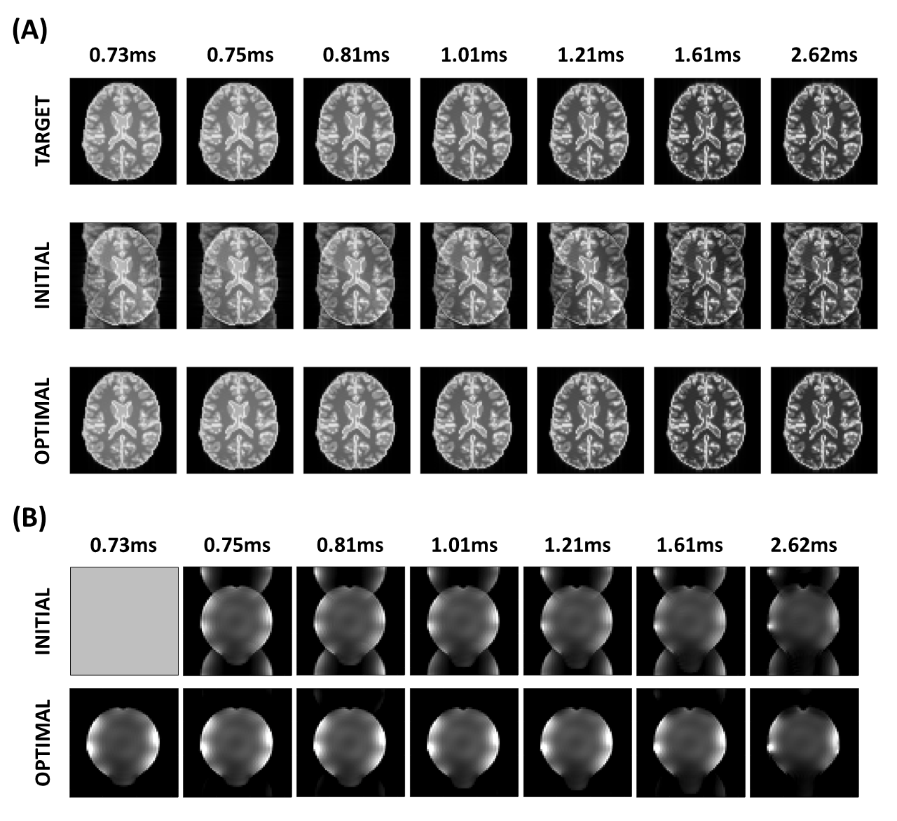
Figure 4: (A) Simulated images using the seven EPI sequences (target) and their predicted distortion after applying the GIRF (initial). NIS optimization removes Nyquist ghosting for all cases (optimal). (B) Reconstructions from data acquired using a spherical water phantom, and the initial and optimal sequences corresponding to the same echo spacings. Improvements are observed across all cases and concur with simulated data in (A). No comparison is possible for 0.73ms as the sequence violates slew rate limits before NIS optimization.
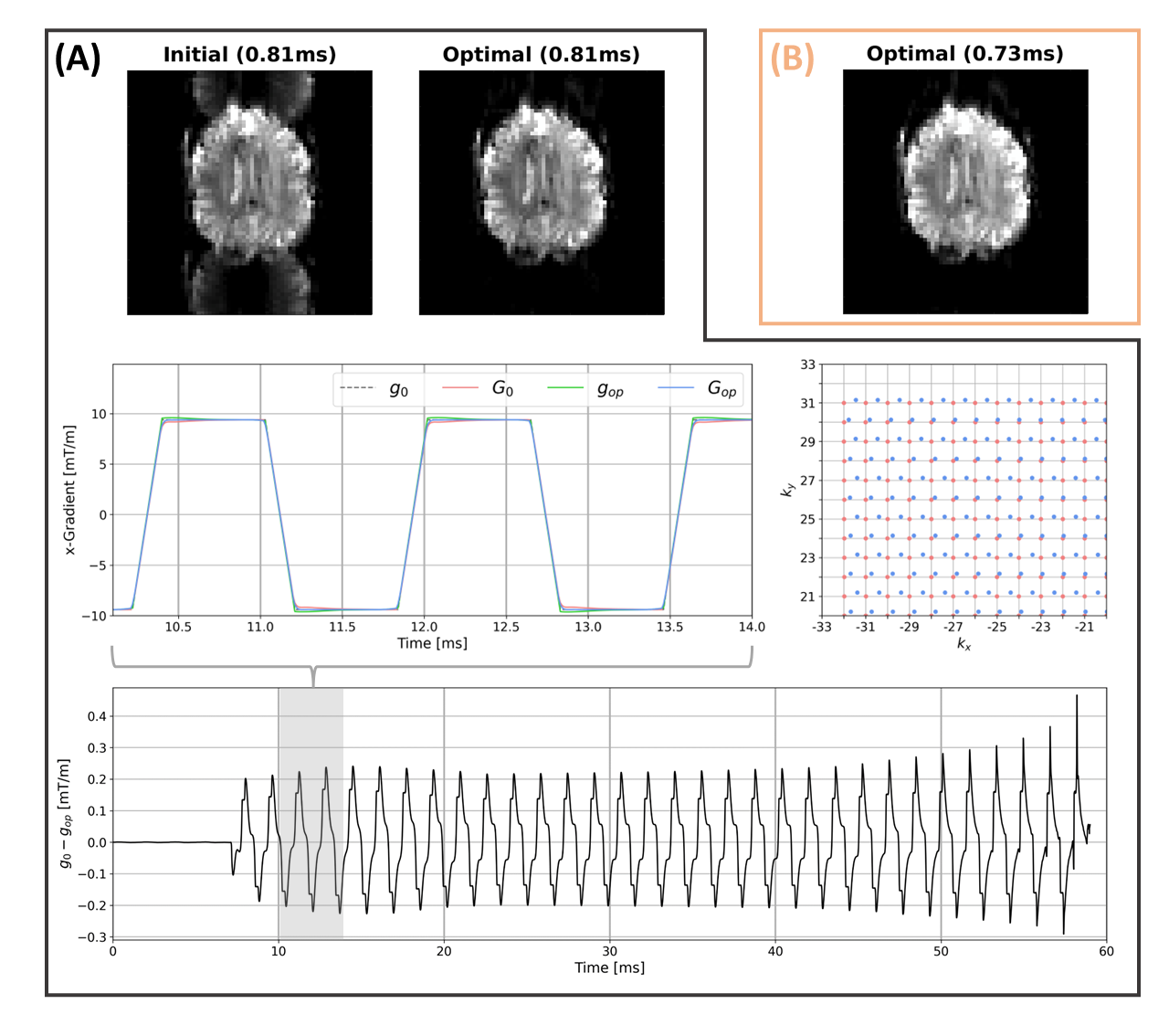
Figure 5: In vivo results obtained from a single healthy volunteer. (A) Results using an inter-echo spacing of 0.81ms. Demanded and realized waveforms are plotted along the middle row for the initial (0) and optimized (op) scenarios across three echoes. Full differences in demanded waveforms are along the bottom row; these go beyond simple pre-emphasis. Corresponding (color-matched) k-space locations are shown on the RHS. (B) NIS optimization succeeds even for a case that previously could not be played on the scanner due to violation of slew rate limits; Nyquist ghosts are removed.