0474
Comparison of Renal ASL Signal-to-noise Ratio and Corticomedullary Contrast between 3T and 5T MRI1School of Biomedical Engineering, ShanghaiTech University, Shanghai, China, 2Central Research Institute, UIH Group, Shanghai, China, 3United Imaging Healthcare, Shanghai, China, 4Application Feature Solution, UIH Group, Shanghai, China
Synopsis
Keywords: High-Field MRI, Arterial spin labelling
Motivation: As the most promising method for measuring tissue perfusion, ASL suffers from low signal-to-noise ratio (SNR), with tagged blood typically causing only few percent of signal difference.
Goal(s): Explore if the use of 5T MRI could lead to higher SNR and CNR for renal ASL than 3T.
Approach: We performed FAIR-EPI on the kidneys of three healthy subjects at 6 inversion times on both 3T and 5T systems. SNR and CNR of difference images were calculated and compared.
Results: SNR at 5T was 10.72±2.81, higher than 7.75±2.65 (P = 0.008) at 3T, and CNR were 9.08±4.08 and 6.53±2.14 (P=0.029), respectively.
Impact: 5T ASL provides difference images with higher SNR and CNR to allow faster acquisition and better corticomedullary differentiation while maintaining comparable image quality.
Introduction
Arterial Spin Labeling (ASL) is a magnetic resonance imaging (MRI) technique for quantification of tissue perfusion. Benefits from non-invasive characteristics, it has a wide application in patients with diseases such as hydronephrosis1. However, because of subtle signal differences, signal-to-noise ratio (SNR) of ASL is significantly low. Recently, 5-tesla (5T) MRI has been approved and gradually put into clinical use. Higher field strength results in higher signal intensity and longer relaxation time2, which may provide potential enhancements for ASL imaging3. The usability of renal ASL scans at 7-tesla has been evaluated4, but no study at 5T has been reported.In this study, three healthy subjects were recruited to have renal ASL scans. We compare the signal-to-noise ratio (SNR) and corticomedullary contrast-to-noise ratio (CNR) between 3T and 5T MRI system and suppose that there may be higher SNR and CNR at 5T.
Methods
All MRI scans were performed on 5T MRI (Jupiter, United Imaging) and 3T MRI (uMR790, United Imaging). Three healthy subjects were recruited. The ASL with flow-sensitive alternating inversion recovery (FAIR) labeling and EPI imaging was performed as following: repetition time (TR) 2800 ms, echo time (TE) 31 ms, scan slice thickness 10 mm, labeling slice thickness 28 mm, inversion time 600, 1000, 1400, 1800, 2200, 2600 ms, FOV 300*220, matrix 147*108, parallel imaging accelerating factor 3. The similar protocol was performed at 3T, except TE 18 ms and accelerating factor 2.We used matlab (2023b, The MathWorks, Inc) for post-processing. Deep learning based kidney segmentation was performed first. Subsequently, rigid and affine registration were employed to correct control and tag images from breathing motion. Difference images were obtained by subtracting tag images from control images.
SNR and CNR were calculated on difference images. Regions of interest (ROIs) were drawn on the background to get the standard deviation of pixels as noise. SNR was defined as mean of cortex and medulla signal divided by noise. To obtain the mean signal, ROIs were drawn over the entire cortex and medulla. CNR was defined as the contrast difference of cortex and medulla divided by noise. To get the contrast, ROIs were drawn on cortex and medulla respectively to obtain the mean signal.
Two-sample t-test was used to compare SNR and CNR between the 3T and 5T MRI. P < 0.05 was considered statistically significant.
Results
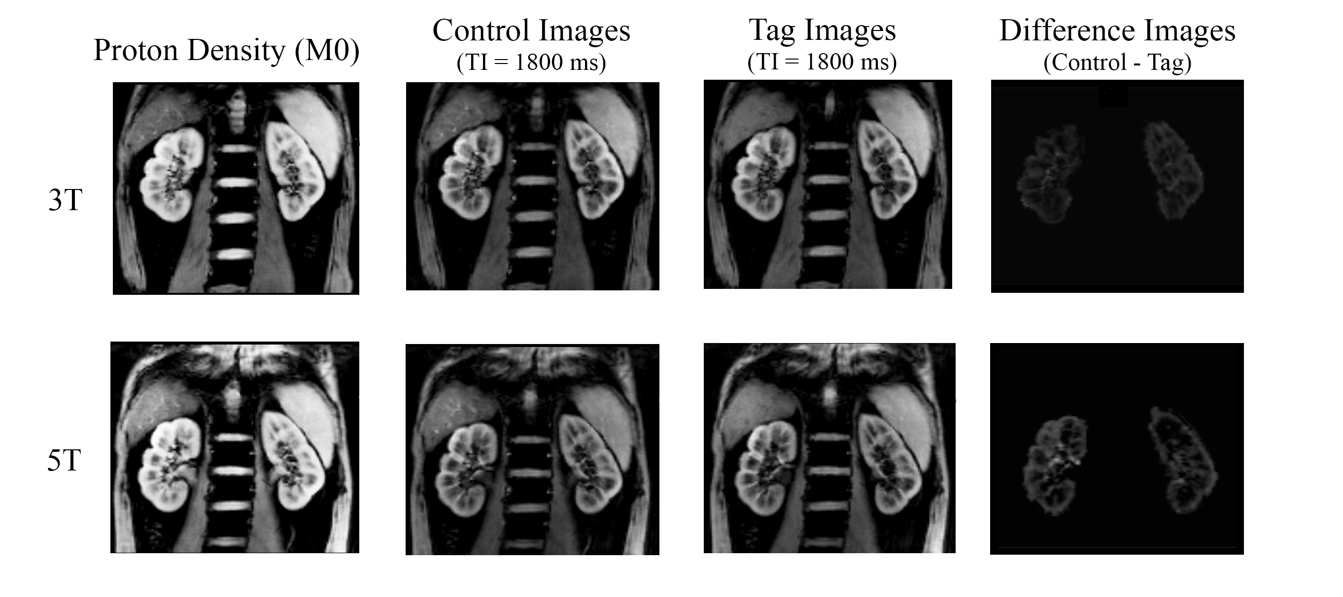
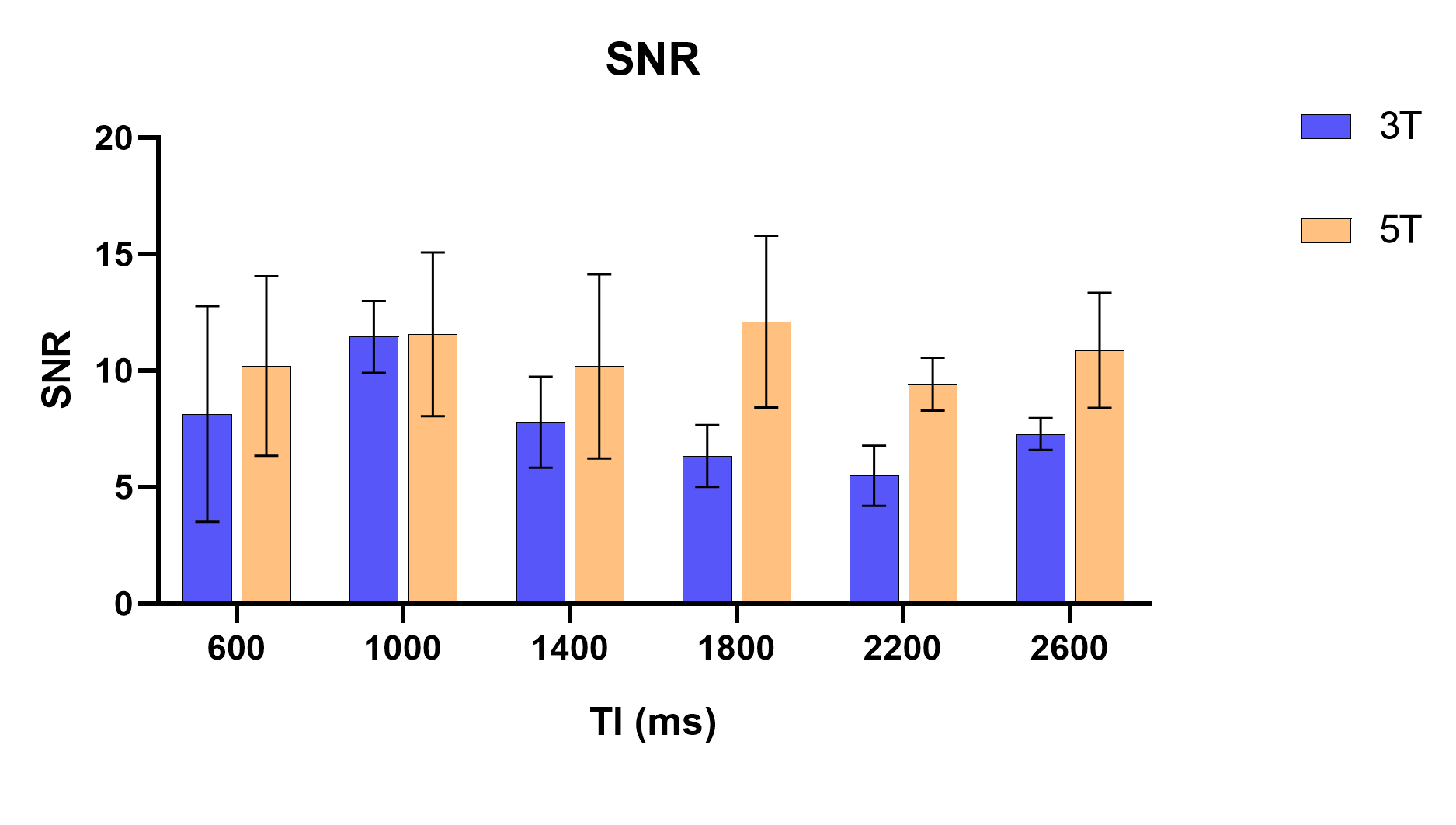
The acquired images and the difference images after post-processing are shown in figure 1.For renal ASL, mean SNR at 5T was 10.72±2.81, higher than 7.75±2.65 (P = 0.008) at 3T. The results of different TIs are shown as figure 2. The highest SNR at 5T was observed at TI=1800 ms, with a value of 12.10±3.01 at 5T, which is 90.8% greater than 6.34±1.08 observed at 3T.
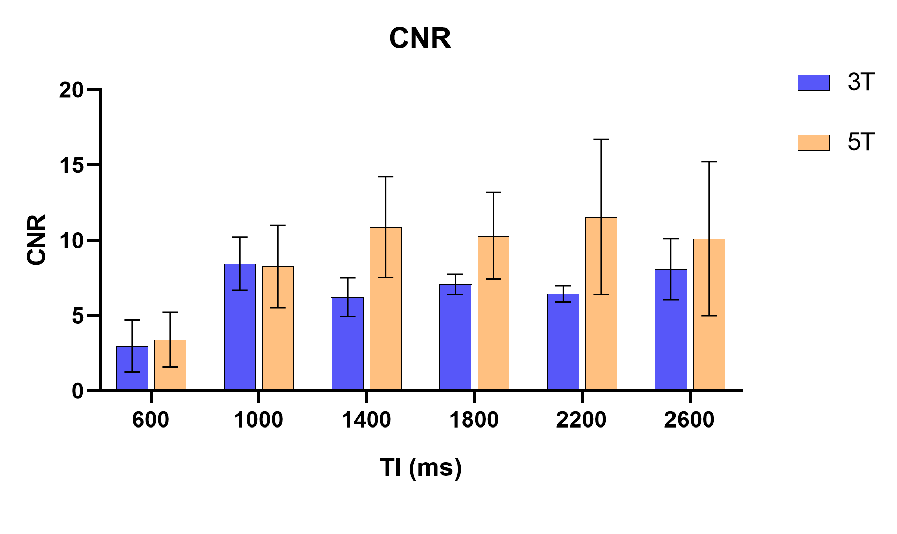
Mean CNR at 5T was 9.08±4.08, higher than 6.53±2.14 (P=0.029) at 3T. CNR of different TIs is illustrated in figure 3. The highest CNR at 5T reached 11.55±4.21 at TI=2200 ms, which is 79.6% greater than 6.43±0.44 observed at 3T.
Discussion
The SNR and CNR of different TIs at 5T system are significantly higher than 3T. The increase in SNR can primarily be attributed to the enhanced signal intensity. Futhermore, labeled blood flows into the imaging slab and reaches its peak at a specific time point, which is equal to the arterial transit time plus the labeling bolus length5. The SNR results suggest that at 3T, the peak may be reached at 1000 ms at 3T and 1800 ms at 5T. This may indicate that 5T MRI offers a wider labeling range and a longer labeling bolus length.As the TI increases, different T1 values of cortex and medulla resulting in an initial increase and subsequent decrease in signal difference, as partially shown in results. The increase of T1 at 5T contributes to a larger signal difference between cortex and medulla, contributing to the improvement of CNR.
Conclusions
Our study demonstrates that the SNR and CNR at 5T MRI system are significantly higher than those at 3T. The improvement in SNR signifies the potential for acquiring fewer images while maintaining comparable image quality, consequently reducing clinical scan time. The notable enhancement in CNR might facilitate the differentiation of the cortex and medulla in perfusion results, especially in patients with hydronephrosis, where the corticomedullary boundary is less distinct. Besides, stability and repeatability remain an area for further investigation. Meanwhile, various homogeneity techniques that have been used for high-field imaging, such as B1+ optimizations, remain to be explored in future research.Acknowledgements
No acknowledgement found.References
1. Bane O, Mendichovszky IA, Milani B, et al. Consensus-based technical recommendations for clinical translation of renal BOLD MRI. Magn Reson Mater Phy. 2020;33(1):199–215.
2. Tsekos NV, Zhang F, Merkle H, Nagayama M, Iadecola C, Kim SG. Quantitative measurements of cerebral blood flow in rats using the FAIR technique: correlation with previous iodoantipyrine autoradiographic studies. Magn Reson Med. 1998;39(4):564–573.
3. Gardener AG, Gowland PA, Francis ST. Implementation of quantitative perfusion imaging using pulsed arterial spin labeling at ultra-high field. Magnetic Resonance in Medicine. 2009;61(4):874–882.
4. Li X, Auerbach EJ, Van de Moortele P-F, Ugurbil K, Metzger GJ. Quantitative single breath-hold renal arterial spin labeling imaging at 7T. Magnetic Resonance in Medicine. 2018;79(2):815–825.
5. Buxton RB, Frank LR, Wong EC, Siewert B, Warach S, Edelman RR. A general kinetic model for quantitative perfusion imaging with arterial spin labeling. Magn Reson Med. 1998;40(3):383-96.
Figures