0450
Acceleration of T2* mapping on an MR Linac using a self-supervised convolutional neural network.1Department of Computing, Imperial College London, London, United Kingdom, 2Joint Department of Physics, The Institute of Cancer Research and The Royal Marsden NHS Foundation Trust, London, United Kingdom, 3FinnBrain Neuroimaging Lab, University of Turku, Turku, Finland, 4The Royal Marsden NHS Foundation Trust, London, United Kingdom, 5Division of Radiotherapy and Imaging, The Institute of Cancer Research, London, United Kingdom
Synopsis
Keywords: MR-Guided Radiotherapy, Quantitative Imaging, Prostate, Radiotherapy, Relaxometry
Motivation: T2* mapping could inform biologically-adaptive MR-guided radiotherapy, but requires improvement in processing time and precision for clinical implementation.
Goal(s): To accelerate intravoxel field inhomogeneity correction and generation of T2* maps.
Approach: We developed a physics-informed self-supervised convolutional neural network for whole volume T2* mapping of complex multi-echo data from an MR Linac. Bias in T2* estimation is accounted for by calculating the additional signal decay from 3D derivatives of the field inhomogeneity map.
Results: Our model generates T2* parameter maps 30% faster than an existing time-efficient algorithm. Resulting T2* maps are less affected by noise compared to the reference.
Impact: Our AI-based algorithm is a step towards integration of whole volume T2* mapping for hypoxia assessment into clinical MR-guided radiotherapy workflows. It could enable real-time mapping of dynamic changes, for example during an oxygen challenge and enable biologically adaptive radiotherapy.
Introduction
The hybrid magnetic resonance linear accelerator (MR Linac) combines MRI with a linear accelerator to deliver precisely targeted radiotherapy to patients with various types of cancer. In addition to high-resolution structural MRI, MR-guided radiotherapy on an MR Linac may also leverage quantitative MRI to provide supplementary information related to treatment response for online treatment adaptation1. One such quantitative MRI parameter is the time constant for the decay in transverse magnetisation; T2*. In this project, we devised a deep convolutional neural network (CNN) that accelerates the computation of voxel-wise T2* parameter maps from 3D multi-echo gradient echo (GE) images acquired on an MR Linac.Methods
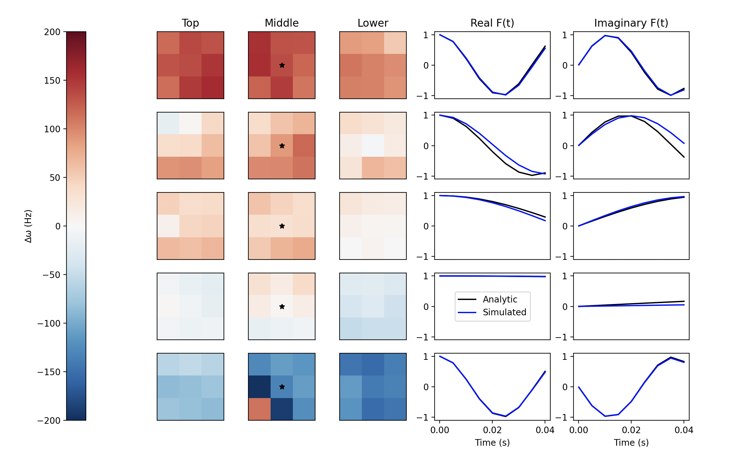
MRI data from 7 participants of the PERMIT trial (NCT03727698) were obtained with written consent and anonymised. Complex 3D multi-echo GE images were acquired using a radial stack-of-stars sequence with golden angle spacing2 on a 1.5T MR Linac (Elekta AB, Stockholm, Sweden) with TE = [5, 10, 15, 20, 25, 30, 35, 40] ms and TR = 48ms, voxel size 1.5×1.5×4mm3. Images were reconstructed using trajectory auto-correction3 and adaptive coil combination4. In total, 47 image volumes (matrix size: 8×32×256×256) were acquired at different treatment fractions, where one patient (7 volumes) was reserved for testing. Images were centrally cropped to a matrix size of (8×22×192×96) and normalised by dividing by the standard deviation of their magnitude. We compared two strategies for estimating the additional signal decay F(t) caused by inhomogeneities in the main magnetic field (∆ω). The first, termed the isochromat summation method5, takes N samples of an interpolated ∆ω-field within the immediate 3x3x3 vicinity of each voxel:$$F(t)=\frac{1}{N}\cdot\sum_{n\in{N}}exp(\Delta\omega_n{it})$$
The second strategy is a closed form approximation that may be derived as continuous generalisation of the isochromat summation method where intravoxel ∆ω variations are assumed to be linear6,7,8:
$$F(t)\approx{exp}(3i\Delta\omega t)\cdot\prod_{j =x,y,z}sinc(grad_j(\Delta\omega)\cdot{t})$$
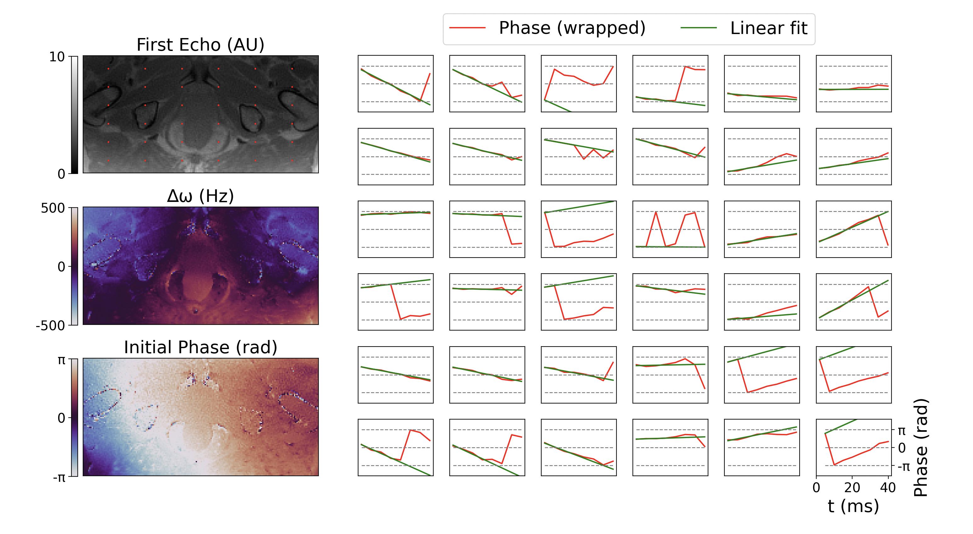
Both strategies rely upon robust estimation of the ∆ω-field which was achieved by unwrapping and fitting a linear model to the phase $$$\phi(t)$$$ of the complex multi-echo data6:
$$\phi(t)=\phi(0)+\Delta\omega{t}$$
Our CNN architecture for volumetric T2* mapping is trained in a physics-informed, self-supervised manner (much akin to previous work9,10) and as such does not require ground truth T2* parameter maps. Our model uniquely takes the concatenated 3D real and imaginary image series as input (matrix size: [16, 22, 192, 96]) and yields 3D parameter maps for T2* = 1/R2* and initial magnetisation, M0 (matrix size: [2, 22, 192, 96]). During model optimisation, these parameter maps and the field-inhomogeneity factor are used to recreate the input volume series using an MR signal model9:
$$S(t) = M_0 \cdot exp(-{R_{2}}^* \cdot{t})\cdot{F(t)}$$
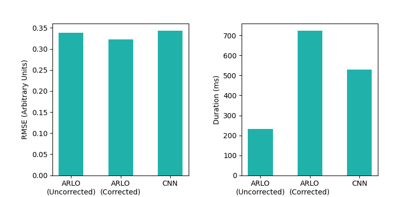
Mean squared error between the input and recreated volumes was used as the loss function. We compared the CNN with ARLO11, a rapid auto-regressive monoexponential fitting algorithm that operates on magnitude data. ARLO was applied both with and without ∆ω-field correction. Algorithms were implemented using Python 3.11 and associated libraries: Pytorch 2.0.1, Numpy 1.21.3, Matplotlib 3.7.1.
Results
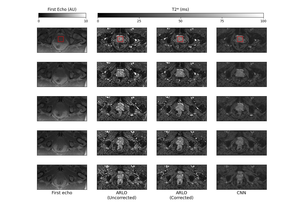
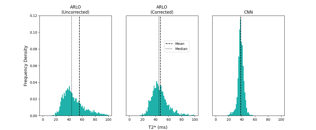
Fig. 1 demonstrates the efficacy of our phase fitting algorithm used to estimate the ∆ω-field. Applying the Numpy.unwrap function consistently rectified phase-wrapping artefacts and permitted robust linear fitting. Fig. 2 is a comparison between our two different strategies for calculating F(t). We observed significant agreement between both strategies in a variety of 3D ∆ω environments and therefore opted to utilise the faster analytic method. Fig. 3 depicts the root mean squared error between the test volumes and reconstructions using ARLO and our CNN. ARLO’s reconstruction error improved slightly if inhomogeneity correction was applied. The CNN’s reconstruction error was comparable to both ARLO implementations. The CNN computed T2* maps 30% faster than ARLO following correction. Fig. 4 is a qualitative comparison between the T2* maps generated using ARLO and the CNN. There is notable agreement regarding the anatomical variation in T2*. ∆ω-corrected ARLO and the CNN appear to be less contaminated with noise with smoother local intensity fluctuations. Fig. 5 offers a quantitative assessment of the three T2* mapping strategies within the prostate. We observed less variance with ∆ω-corrected ARLO and the CNN. ∆ω-corrected ARLO and the CNN also had substantially reduced mean T2*s within the prostate.Conclusions
We devised an algorithm that rapidly estimates the additional signal loss caused by magnetic field inhomogeneities in complex multi-gradient echo images. The effectiveness of our ∆ω-gradient based technique is evidenced by reduced residuals of monoexponential fitting with ARLO following correction. Further, we demonstrated the use of a self-supervised CNN for rapid 3D T2* mapping. The reconstruction error for parameter maps generated using the CNN was comparable to that of ARLO and is expected to improve with more training.Acknowledgements
This research was supported by the CRUK Convergence Science Centre at The Institute of Cancer Research, London, and Imperial College London (A26234).
The Institute of Cancer Research and The Royal Marsden NHS Foundation Trust are members of the Elekta MR-Linac Research Consortium. We acknowledge research support from Elekta and Dave Higgins (Philips MR) for providing MR source code, research licences, and support.
References
1. Bano W, Holmes W, Goodburn R, Golbabaee M, Gupta A, Withey S, et al. Joint radial trajectory correction for accelerated T2* mapping on an MR-Linac. Medical Physics. 2023 May. Available from: doi.org/10.1002/mp.16479
2. S. Winkelmann, T. Schaeffter, T. Koehler, H. Eggers and O. Doessel, "An Optimal Radial Profile Order Based on the Golden Ratio for Time-Resolved MRI," in IEEE Transactions on Medical Imaging, vol. 26, no. 1, pp. 68-76, Jan. 2007, doi: 10.1109/TMI.2006.885337.
3. Ianni, J.D. and Grissom, W.A. (2016), Trajectory Auto-Corrected image reconstruction. Magn. Reson. Med., 76: 757-768. https://doi.org/10.1002/mrm.25916
4. Walsh, D.O., Gmitro, A.F. and Marcellin, M.W. (2000), Adaptive reconstruction of phased array MR imagery. Magn. Reson. Med., 43: 682-690. https://doi.org/10.1002/(SICI)1522-2594(200005)43:5<682::AID-MRM10>3.0.CO;2-G
5. Shkarin P, Spencer RGS. Direct simulation of spin echoes by summationof isochromats. Concepts in Magnetic Resonance. 1996;8(4):253-68. Availablefrom: doi.org/10.1002/(SICI)1099-0534(1996)8:4<253::AID-CMR2>3.0.CO;2-Y
6. Yablonskiy DA, Sukstanskii AL, Luo J, Wang X. Voxel spread function method for correction of magnetic field inhomogeneity effects in quantitative gradient-echo-based MRI. Magn Reson Med. 2013 Nov;70(5):1283-92.
7. Koch KM, Rothman DL, de Graaf RA. Optimization of static magnetic field homogeneity in the human and animal brain in vivo. Prog Nucl Magn Reson Spectrosc. 2009Feb;54(2):69-96
8. Lam F, Sutton BP. Intravoxel B0 inhomogeneity corrected reconstruction using a low-rank encoding operator. Magnetic Resonance in Medicine;84(2):885-94. Available from: https://onlinelibrary.wiley.com/doi/abs/10.1002/mrm.28182
9. Torop M, Kothapalli SVVN, Sun Y, Liu J, Kahali S, Yablonskiy DA, et al. Deep learning using a biophysical model for robust and accelerated reconstruction of quantitative, artifact-free and denoised images. Magnetic Resonance in Medicine. 2020;84(6):2932-42. Available from: doi.org/10.1002/mrm.28344
10. Troelstra MA, Van Dijk AM, Witjes JJ, et al. Self-supervised neural network improves tri-exponential intravoxel incoherent motion model fitting compared to least-squares fitting in non-alcoholic fatty liver disease. Front Physiol. 2022;13:942495. Published 2022 Sep 6. doi:10.3389/fphys.2022.942495
11. Pei M, Nguyen TD, Thimmappa ND, Salustri C, Dong F, Cooper MA, et al. Algorithm for fast monoexponential fitting based on Auto-Regression on Linear Operations (ARLO) of data. Magnetic Resonance in Medicine. 2015;73(2):843-50. Available from: doi.org/10.1002/mrm.25137
Figures