Introduction

fMRI can detect fluid flow in the brain with high sensitivity and temporal resolution ¹, but does not yield quantitative velocity measures, which are important for clinical and neuroscientific applications. Prior work developed a physics-based forward model for the relationship between dynamic flow velocity and flow-enhanced fMRI signals ^2,3. This model simulates fMRI inflow signals using velocity, suggesting the model could in principle be inverted to infer velocities from fMRI data. Here, we designed a neural network to learn the inverse mapping between fMRI inflow signals and velocities. This work enables direct quantification of time-dependent flow velocity from fMRI data.

Methods

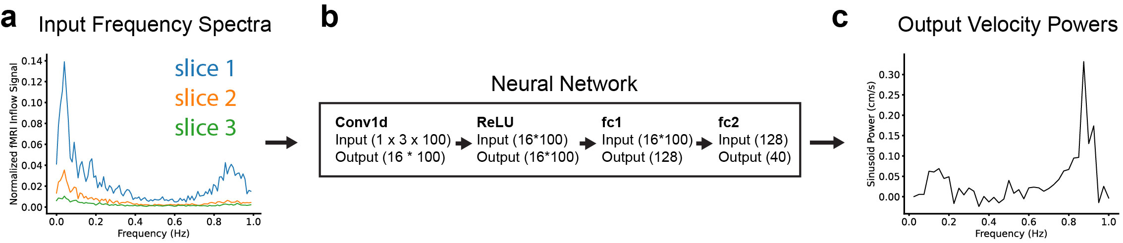
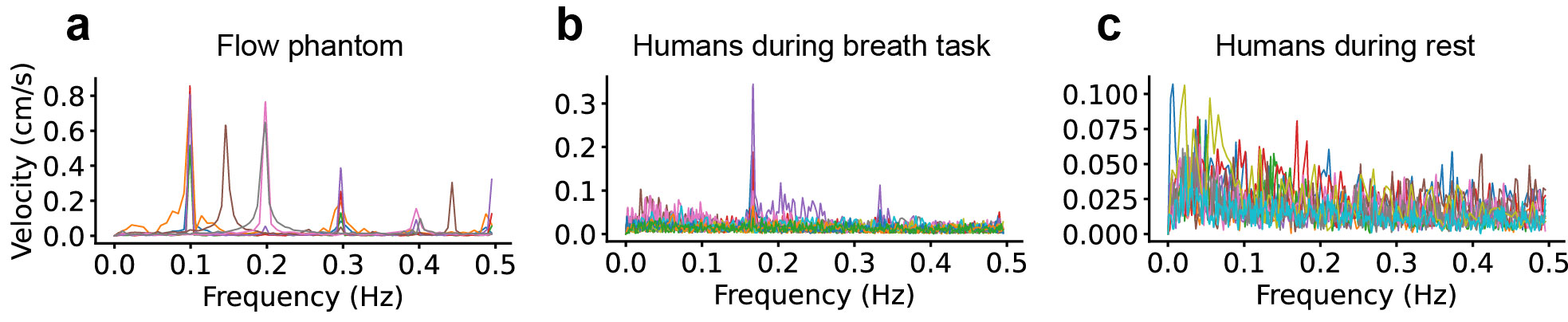
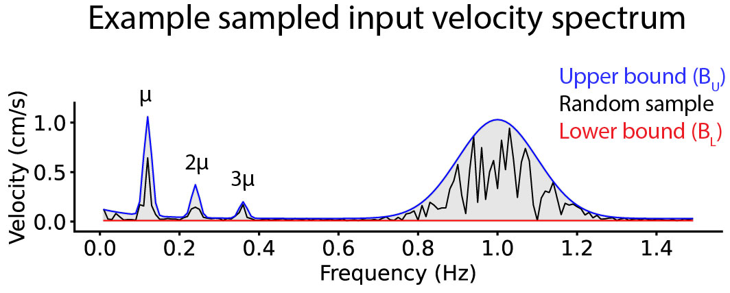
Our approach is to analyze signals in the frequency domain so we can extract information about velocities across the full range of oscillatory dynamics in the flow signal. The neural network (Fig.1) takes fMRI inflow signal spectra as input and outputs powers in cm/s. We trained the neural network on simulated data generated by the physics-based forward model, which takes an input velocity V_input, and predicts the resulting fMRI inflow signal. Each V_input is a sum of N_f sinusoids defined as $$$V_{input}=\sum_{i=1}^{N_f}V_i\sin(2\pi f_it)$$$, (V_i=power; f_i=frequencies, t=time). We used N_f=40 where frequencies ranged between 0.025-1Hz, and powers were sampled from a distribution based on magnitudes observed in real velocity data measured via phase contrast (Fig.2). We defined the sampling bounds such that each f_i is randomly assigned a V_i between B_L(f_i) and B_U(f_i), where B_L(f) and B_U(f) are frequency-dependent curves defining the lower and upper velocity bounds. B_L is a constant 0.02 cm/s, and B_U was defined as
$$B_U(f)=\frac{1}{8}e^{-10f}+(e^{-\frac{1}{2}(\frac{f-\mu}{0.01})^2}+\frac{1}{3}e^{-\frac{1}{2}(\frac{f-2\mu}{0.01})^2}+\frac{1}{6}e^{-\frac{1}{2}(\frac{f-3\mu}{0.01})^2})+e^{-\frac{1}{2}(\frac{f-1}{0.1})^2}.$$ The first term in B_U represents the exponential shape of the slow frequency region (<0.1Hz) observed in our human data (Fig.2b/c), the second term represents dynamics from a breathing frequency µ (randomly selected between 0.1-0.3Hz for each sample) including harmonics at 2µ and 3µ, and the third term accounts for cardiac fluctuations which we could not resolve with our phase contrast protocol (due to aliasing) so we used a gaussian centered at 1Hz. Fig.3 shows one example curve sampled between B_L and B_U, with a randomly chosen µ.
We performed experiments on a flow phantom and in humans during paced breathing, since CSF flow is driven by breathing ⁴. The phantom consisted of a syringe pump that controlled water flow in a tube routed into the scanner. To produce oscillatory flows using the pump, we set the flow to oscillate at either 0.1, 0.15, or 0.2 Hz. Eight human participants provided informed written consent and all experimental procedures were approved by the Institutional Review Board. Experiments were performed on a 3T Siemens Prisma scanner with a 64-channel head coil. Anatomical images were acquired with a 1 mm isotropic multi-echo MPRAGE anatomical scan. fMRI inflow signals were measured using gradient-echo fMRI (TR=0.504s, TE=0.03s, 2.5mm isotropic, MB=3, 21 slices , FA=45). Phase contrast runs used a TR=1.01s, 2.5mm isotropic voxels, single-slice, VENC=6cm/s. We acquired human data during runs of paced breathing at 0.167 Hz and separate runs of rest. For all human and phantom experiments, we acquired fMRI and phase contrast data for each condition. CSF flow was extracted as the mean signal in the fourth ventricle using an anatomically-based ROI.

Results

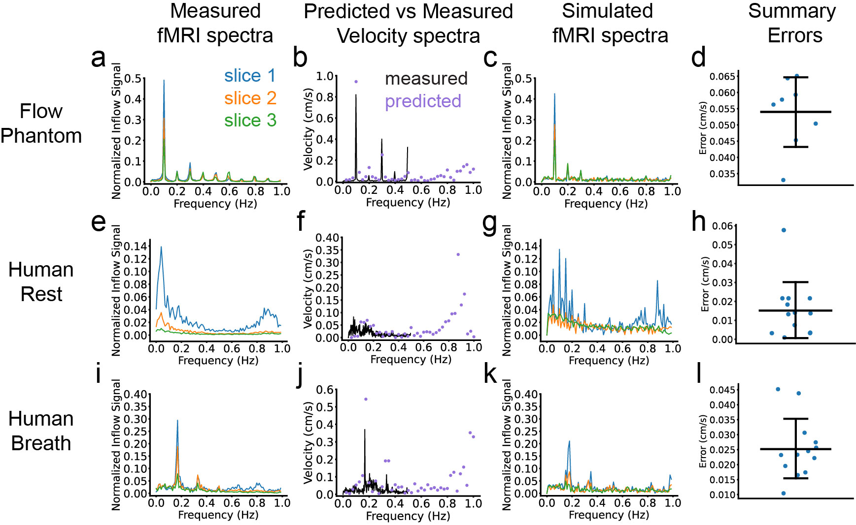
The neural network was trained on 250,000 simulated samples. The trained model accurately predicted flow velocity using measured fMRI data as input, with mean errors of 0.054 ± 0.01, 0.015 ± 0.014, and 0.025 ± 0.0095 cm/s for phantom, human resting state, and human paced breathing data, respectively (Fig.4d,h,l). Representative examples show that the network effectively generalized to infer velocity in real datasets (Fig. 4). Furthermore, we confirmed model performance by using the forward model on the predicted velocities, which generated fMRI timeseries that were well matched to the data (Fig.4). Additionally, this model enabled us to extract information about velocity dynamics in the cardiac band (purple dots >0.8Hz in Fig.4b,f,g) which was previously not available from the phase contrast data due to its lower sampling rate.

Discussion

Here, we designed a neural network framework used to directly quantify flow velocity from fMRI signals alone. Our approach leveraging the physics-based forward model to generate training data is flexible because any dynamics can be learned by adjusting B_L and B_U. Although we used phase contrast data to design the bounds, phase contrast data are not required to apply the model. This work is a significant advancement in flow imaging because it enables quantitative assessments of flow using fMRI, which already provides high sensitivity and temporal resolution as well as the ability to simultaneously monitor hemodynamics.

Acknowledgements

This work was supported by National Institutes of Health grants NIH U19NS128613 and R01AG070135

References

1. Fultz, N. E., Bonmassar, G., Setsompop, K., Stickgold, R. A., Rosen, B. R., Polimeni, J. R., & Lewis, L. D. (2019). Coupled electrophysiological, hemodynamic, and cerebrospinal fluid oscillations in human sleep. Science, 366(6465), 628-631.

2. Ashenagar, B., Gomez, D., Lewis, L. Modeling inflow effects in fast fMRI to quantify fluid flow. Proc. Intl. Soc. Mag. Reson. Med. 31 (2023). Abstract #1174

3. Gao, J. H., Miller, I., Lai, S., Xiong, J., & Fox, P. T. (1996). Quantitative assessment of blood inflow effects in functional MRI signals. Magnetic resonance in medicine, 36(2), 314-319.

4. Dreha-Kulaczewski, S., Joseph, A. A., Merboldt, K. D., Ludwig, H. C., Gärtner, J., & Frahm, J. (2017). Identification of the upward movement of human CSF in vivo and its relation to the brain venous system. Journal of Neuroscience, 37(9), 2395-2402.