0264
3D MR Fingerprinting for Prostate at 0.55 T1Department of Radiology, University of Michigan, Ann Arbor, MI, United States, 2Department of Biomedical Engineering, Univeristy of Michigan, Ann Arbor, MI, United States
Synopsis
Keywords: Prostate, Prostate, prostate cancer, 0.55 T, low field, MRF, fingerprinting, synthesized contrast
Motivation: 0.55 T MRI scanners have lower fields inhomogeneities and bigger bore size when compared to higher fields, allowing to scan larger body habitus patients, and to perform MRI-guided biopsies.
Goal(s): To generate 1x1x3 mm3 T1 and T2 maps of the prostate and T1 and T2 weighted images with improved contrast from MRF at 0.55 T.
Approach: We use a 3D MRF-FISP sequence with Stack of Spirals acquisition and a low-rank denoising method.
Results: We show T1 and T2 maps and T1 and T2 weighted images and report on values for the prostate NPZ and NTZ of 5 subjects and for a biopsy-confirmed lesion.
Impact: Implementing prostate MR Fingerprinting at 0.55 T, allows multiparametric quantitative assessment of the gland while gaining advantages that 0.55 T scanners offer respect to higher field ones. This includes lower fields inhomogeneities, bigger bore size and a lower equipment cost.
Introduction
This study aims to provide a fast quantitative imaging approach for prostate cancer using a commercial 0.55 T MRI scanner. Low-field has gained significant interest recently due to its potential to improve the accessibility of MRI [1, 2]. However, low SNR and slew rates and gradient amplitudes constraints create challenges in generating images with high spatial resolutions for small lesion detection. Altered contrast properties at 0.55 T compared to 3 T may also reduce the visibility of prostate lesions. We demonstrated the feasibility of quantifying T1 and T2 at a spatial resolution of 1×1×3 mm3 using a 3D MR Fingerprinting (MRF) approach and generating images with enhanced contrast using these maps to improve the conspicuity of the lesion.Methods
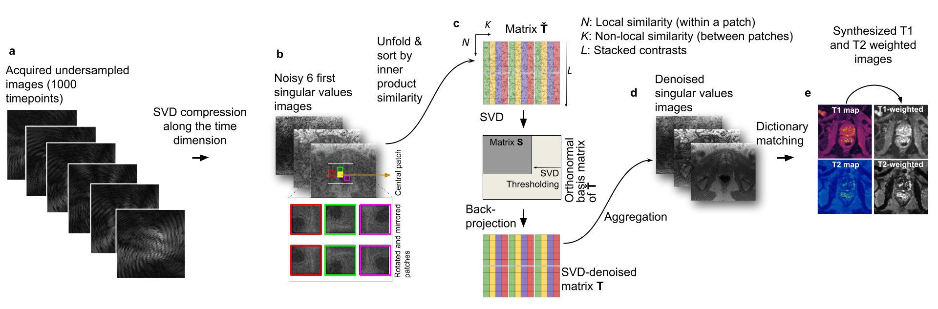
Acquisition: An MRF acquisition with stack-of-spirals trajectory was implemented on a 0.55 T scanner (Magnetom Free.Max, Siemens Hearlthineers, Erlangen, Germany). To satisfy gradient constraints, the duration of the spiral was extended to 12.6 ms with a FOV of 400 mm. 1000 time points were acquired with variable flip angles, leading to a scan time of 9 minutes for 26 partitions.Reconstruction and denoising: MRF time series was first SVD-compressed to 6 coefficient images (Fig. 1a). To improve the SNR, a low-rank denoising algorithm [3] was applied as shown in Fig. 1b. The algorithm approximates noise-free images by low-rank thresholding a matrix formed with patches that have similar image structures. Specifically, for each 3x3 pixels patch, twenty other patches were selected by sorting their inner products with this patch (Fig. 1c) to group similar structures. Additional patches were created by rotating and mirroring these patches [3]. Denoising was achieved by keeping the first 6 coefficients (91 % of information) and refolding and averaging the matrix (Fig. 1d). T1 and T2 maps (Fig. 1e) were generated by matching the denoised images with a pre-calculated MRF signal dictionary.
Lesion-specific contrast-weighted images: Inversion recovery (IR) T1 and spin-echo (SE) T2 weighted images were calculated using the denoised maps (Fig. 1e).
Phantom and In-vivo experiments: T1 and T2 estimations of the proposed methods were validated using the NIST phantom [4]. Five healthy subjects were scanned at 0.55 T and 3 T. In addition, a patient with suspicion of prostate cancer, undergoing an MRI-guided biopsy at 0.55T with resultant pathology confirmed clinically significant cancer (Gleason score of 3+4=7) was scanned.
Results
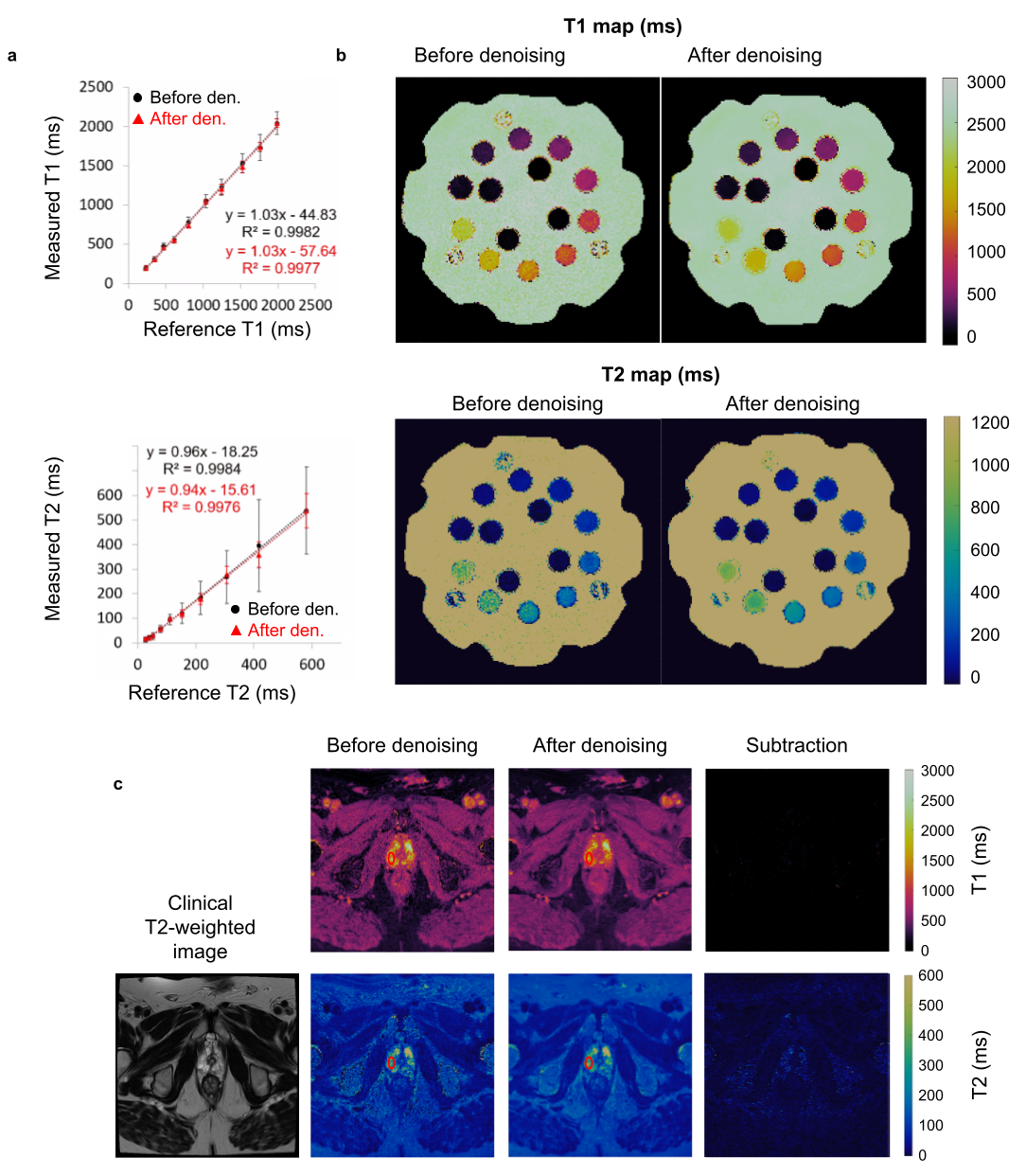
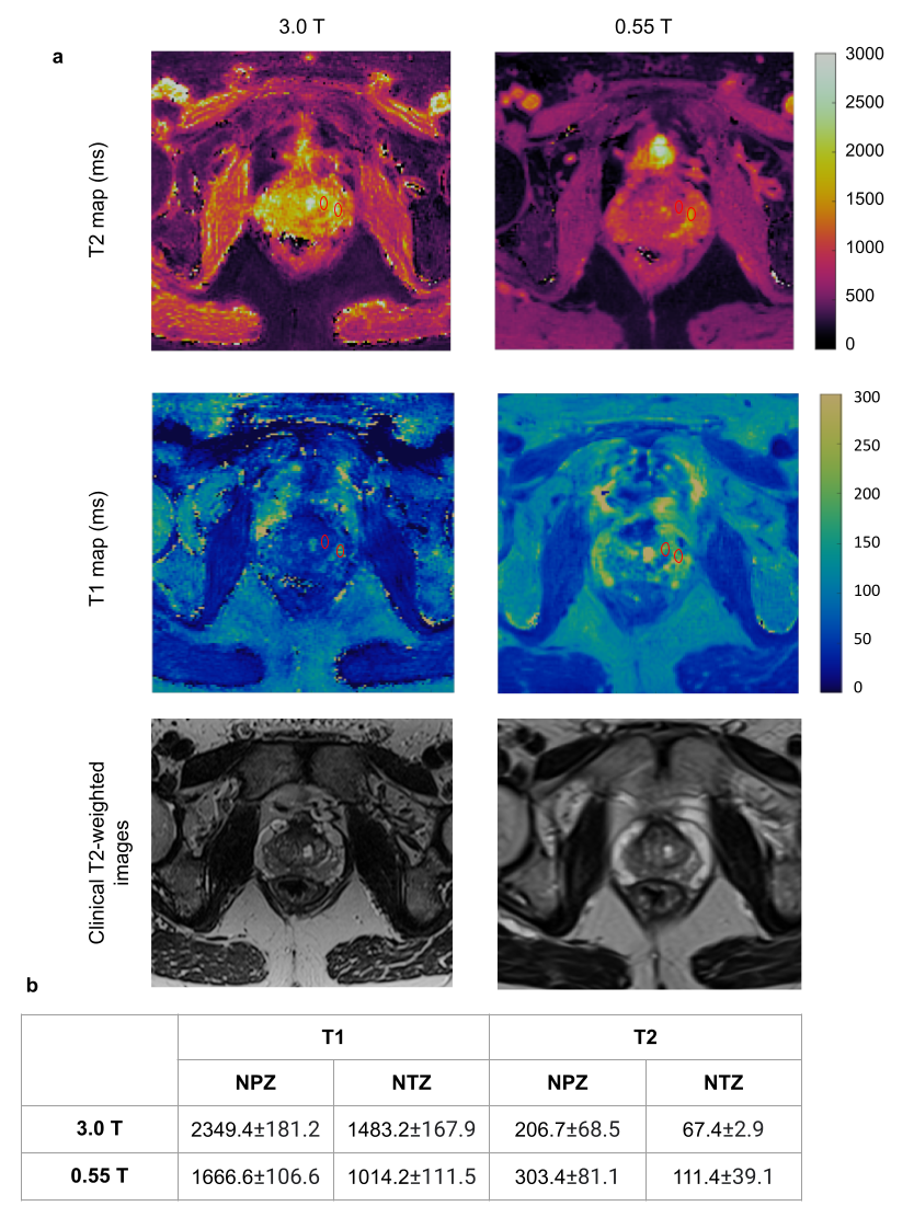
In Fig. 2a, T1 and T2 values estimated using MRF with and without using the denoising algorithm are compared to gold standard T1 and T2 values. T1 and T2 maps are shown in Fig. 2b, demonstrating that accurate T1 and T2 values can be obtained using the proposed MRF acquisition at 0.55 T. The proposed denoising algorithm improves the precision across all T1 and T2 values by reducing their standard deviations. T1 and T2 maps from a healthy subject are shown before and after applying denoising in Fig. 2c, as well as subtraction maps. T1 and T2 values for an ROI drawn in the normal-appearing peripheral zone (NPZ) (highlighted in red) are respectively 1882±281 ms, 447±271 ms before and 1730±151 ms, 400±63 ms after denoising. Denoised T1 and T2 values fall within the SD of the non-denoised values.Fig. 3 compares T1 and T2 maps acquired at 0.55 T and 3 T from one healthy subject. T1 and T2 values of the NPZ and normal-appearing transition zone (NTZ) of 5 subjects were reported.
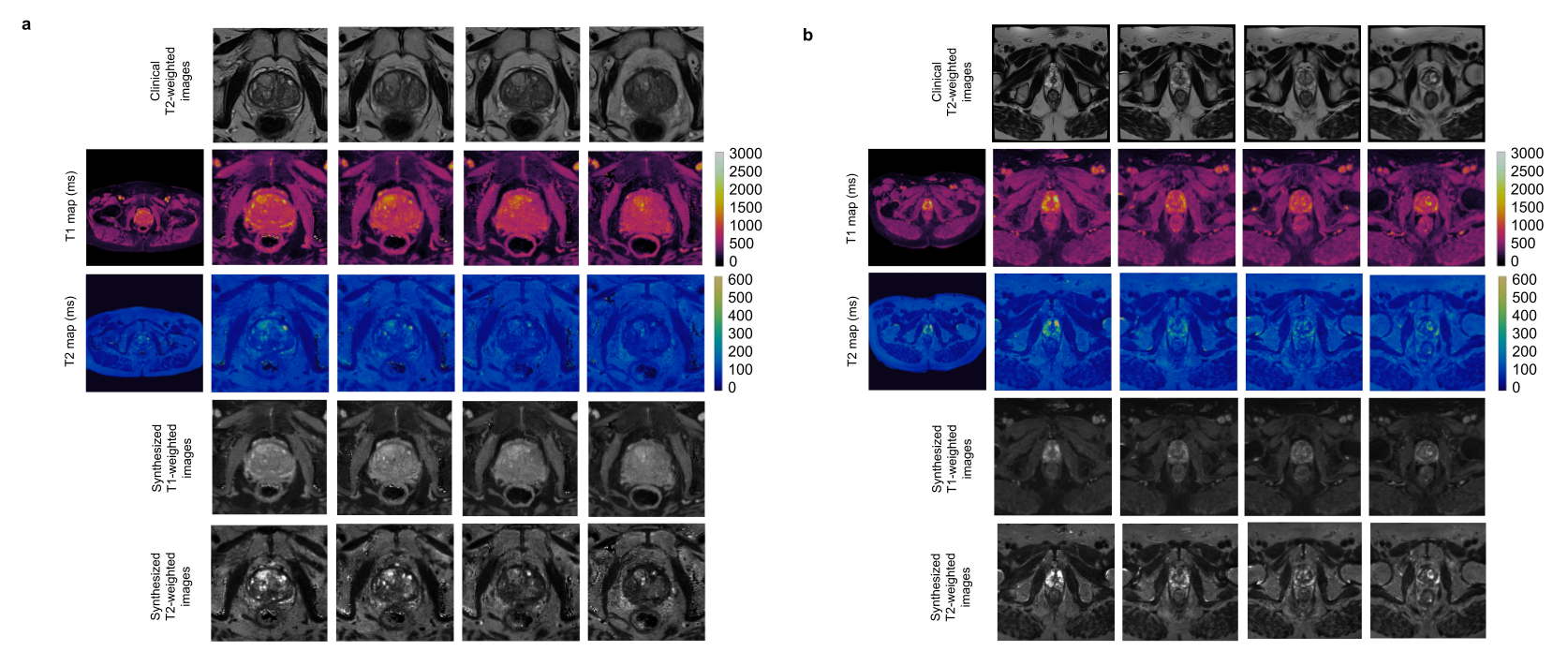
Fig 4 shows T1, T2 maps and calculated T1-weighted and T2-weighed images from two healthy subjects.
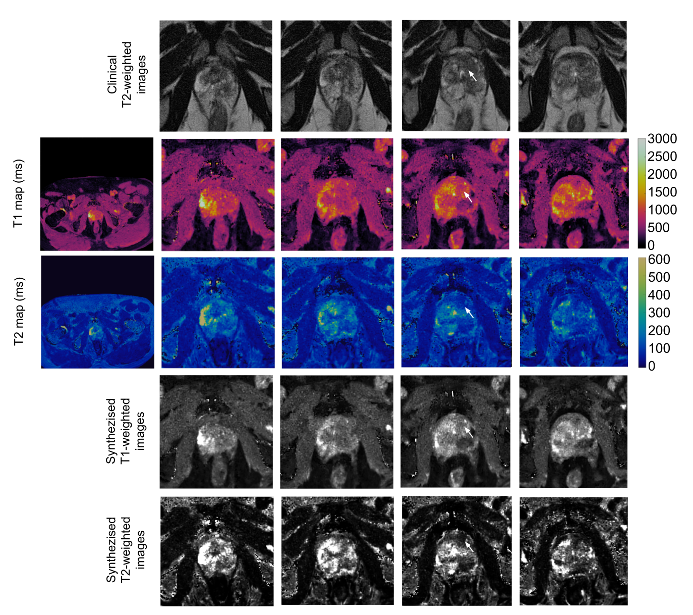
Fig. 5 shows T1 and T2 maps from a patient with a confirmed TZ lesion (Gleason score 7, T1 = 643±181 ms, T2 = 69±22 ms) and a large area of prostatitis in the left posterior peripheral zone. T1 and T2-weighted images were generated to improve the conspicuity of the lesion by adjusting contrasts based on T1 and T2 values of the tumor and the surrounding tissue. CNR of the lesion was 1.39 in clinical T2-weighted images and 1.90 and 2.01 for our calculated T1 and T2-weighted images.
Conclusion and Discussion
A 3D MRF acquisition with a denoising algorithm was proposed to generate high-resolution T1 and T2 maps of the prostate gland on a commercial 0.55T scanner. Contrast-enhanced T1 and T2-weighted images were generated from the MRF T1 and T2 maps in attempt to improve the visualization of the tumor. Our initial results suggest that this proposed approach has the potential to provide high-quality quantitative maps for characterizing prostate cancer as well as tailored contrast-weighed images for better tumor visualization. Additional validation experiments in patients with suspicion of cancer are underway.Acknowledgements
Support for this study was provided by NIH grants R37CA263583 and R01CA208236, and Siemens Healthcare.References
1. Runge, V.M., & Heverhagen, J. T. The clinical utility of magnetic resonance imaging according to field strength, specifically addressing the breadth of current state-of-the-art systems, which include 0.55 Y, 1.5 T, 3 T and 7 T. Investigative Radiology. 2022; 57(1) 1-12.
2. Campbell-Washburn, A. E., Jiang, Y., Körzdörfer, G., Nittka, M., & Griswold, M. A. Feasibility of MR fingerprinting using a high-performance 0.55 T MRI system. Magnetic Resonance Imaging. 2021; 81, 88-93.
3. Cruz, G., Liu, Y., Cummings, E., Hamilton, J., Gulani, V. and Seiberlich, N. Improved T1, T2 and PDFF mapping with rosette MRF using virtual-coil + low-rank + patch-based regularization, Proceedings of the International Society of Magnetic Resonance in Medicine, Toronto. 2023.
4. Keenan, K. , Stupic, K. , Boss, M. , Russek, S. , Chenevert, T. , Prasad, P. , Reddick, W., Zheng, J. , Hu, P. and Jackson. Comparison of T1 measurement using ISMRM/NIST system phantom, Proceedings of the International Society of Magnetic Resonance in Medicine, Singapore. 2016.
5. Fajardo, JE., Lavrova, A., Gulani, V. and Jiang, Y. 3D High Resolution MR Fingerprinting for prostate cancer, Proceedings of the International Society of Magnetic Resonance in Medicine, Toronto. 2023.
Figures