0183
Artifact free Projection onto Dipole Fields via a Generalized Frequency-domain Discrete Dipole Kernel1School of Electrical Engineering, Pontificia Universidad Catolica de Valparaiso, Valparaiso, Chile, 2Pontificia Universidad Catolica de Chile, Santiago, Chile, 3Department of Medical Physics and Biomedical Engineering, University College London, London, United Kingdom, 4SJTU-Ruijin-UIH Institute for Medical Imaging Technology, Shanghai Jiaotong University School of Medicine, Shanghai, China, 5School of Psychological and Cognitive Sciences; Beijing Key Laboratory of Behavior and Mental Health; IDG/McGovern Institute for Brain Research; Peking-Tsinghua Center for Life Sciences, Peking University, Beijing, China
Synopsis
Keywords: Susceptibility/QSM, Quantitative Susceptibility mapping, Background field removal
Motivation: Overcoming striping artifacts in the background removal step is a common challenge, especially in non-orthogonal (oblique) B0 field orientations.
Goal(s): Develop a robust solution to eliminate striping artifacts while improving the accuracy of QSM images.
Approach: We introduce a novel approach, employing a generalized discrete kernel to suppress striping artifacts generated by the Projection onto Dipole Fields method.
Results: Our approach successfully addresses striping artifacts and enhances the accuracy of PDF solutions, even at non-orthogonal B0 field angles, promising artifact-free results.
Impact: Our work promises to benefit the EMTP community by providing a more robust solution for addressing striping artifacts. This can lead to improved diagnostic accuracy and higher-quality imaging, ultimately enhancing patient care and advancing MRI technology.
INTRODUCTION
The phase in Gradient Echo MRI acquisitions contains the magnetic field's local deviations relative to the main magnetic field. These deviations encompass field inhomogeneities and tissue magnetization fields. Quantitative Susceptibility Mapping (QSM) is an ill-posed inverse problem, where susceptibility sources are represented as magnetic dipoles, requiring a deconvolution to pinpoint these sources from the magnetic field. As the total magnetic field is dominated by the magnetization of air-tissue interfaces and background sources (outside the region of interest, ROI), QSM requires to disentangle local magnetizations from background fields. Given that background fields are harmonic fields, numerous methods have been devised to separate them1 from local fields, which are not harmonic. Among these methods, the Projection onto Dipole Fields (PDF)2 method stands out as a popular and robust choice. In essence, PDF tackles an inverse problem similar to QSM, but estimating susceptibility sources outside a ROI ($$$\chi_{\text{out}}$$$):$$\arg\min_{\chi_{\text{out}}}\left\|W\left(F^HDF\chi_{\text{out}}-\phi_{\text{total}}\right)\right\|_2^2\;\;\;\;\;Eq.1.$$
where $$$D$$$ is the dipole kernel, $$$F$$$ the Fourier transform and $$$F^H$$$ its inverse. $$$\phi_{total}$$$ is the total magnetization field. If B0 is along the z axis, D has a simple expression3,4: $$$1/3–k_z^2/k^2$$$, being $$$k_i$$$ the Fourier domain indexes.
More generally, for $$$\vec{H}_0$$$ the main field in an arbitrary direction and $$$widehat{b}_0$$$ the unitary vector pointing in the direction of $$$B_0$$$, $$$\nabla^2\Phi_{\text{obj}}=\vec{H}_0\cdot\vec{\nabla}\chi$$$ (with $$$\Phi_{\text{obj}}$$$ the magnetic scalar potential of the object $$$h_{obj}$$$) and $$$h_{\text{obj},\widehat{b}_0}=-\vec{\nabla}\Phi_{\text{obj}}\cdot\widehat{b}_0$$$, then the continuous kernel becomes:
$$D_{\widehat{b}_0}=\frac{1}{3}-\frac{\left(\widehat{b}_0\cdot \vec{k}\right)^2}{k^2}\;\;\;\;\;Eq.2.$$
This enables estimating QSM and PDF with B0 field in any orientation. Unfortunately, PDF at non-orthogonal angulations with respect to the B0 field has been plagued by striping artifacts5. These artifacts manifest as checkerboard patterns which are primarily originated by the discrete Fourier Transformation's limitations and the use of the continuous dipole kernel in the frequency domain. As highlighted by Kiersnowski5 and Dixon6, these striping artifacts can be reduced by employing the Green’s function – the dipole kernel defined in the spatial domain7:
$$D_{s,\widehat{b}_0}=\frac{3\left(\widehat{b}_0\cdot\vec{r}\right)^2-r^2}{4\pi{r^5}}\;\;\;\;\;Eq.3.$$
Regrettably, the use of this function in PDF introduces new challenges, particularly degrading low-frequency components and generating large, smooth field residuals or shadowing artifacts. A common workaround is to rotate the acquired image to eliminate the B0 field's angulation, but this introduces blurring due to interpolation. In this work, we propose an innovative method to effectively reduce striping artifacts while enhancing the accuracy of PDF solutions.
METHODS
Milovic8 proposed a discretized dipole kernel in the frequency domain using finite differences and the discrete Fourier Transform to decouple operations between voxels. Similarly, if we take the gradient operators9,10 $$$E_i=1-e^{2\pi{j}\frac{k_i}{N_i}}$$$, with $$$N_i$$$ the length in a given axis $$$i=x,y,z$$$, then Eq. 2 becomes the generalized discrete kernel:$$D_{d,\widehat{b}_0}=\frac{1}{3}-\frac{\left\langle{\widehat{b}_0}\cdot\vec{E},{\widehat{b}_0}\cdot\vec{E}\right\rangle}{\left\langle\vec{E},\vec{E}\right\rangle}\;\;\;\;\;Eq.4.$$
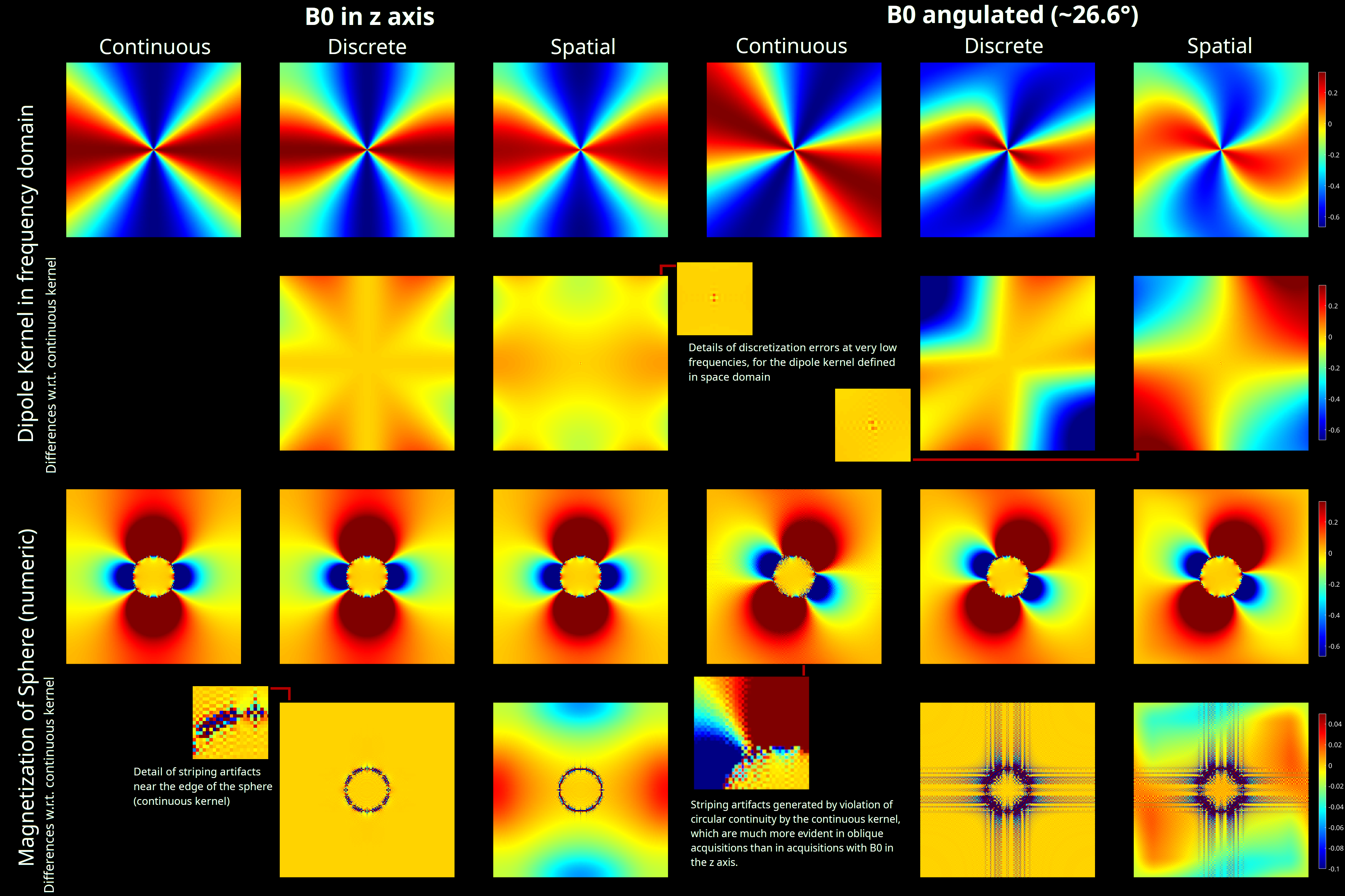
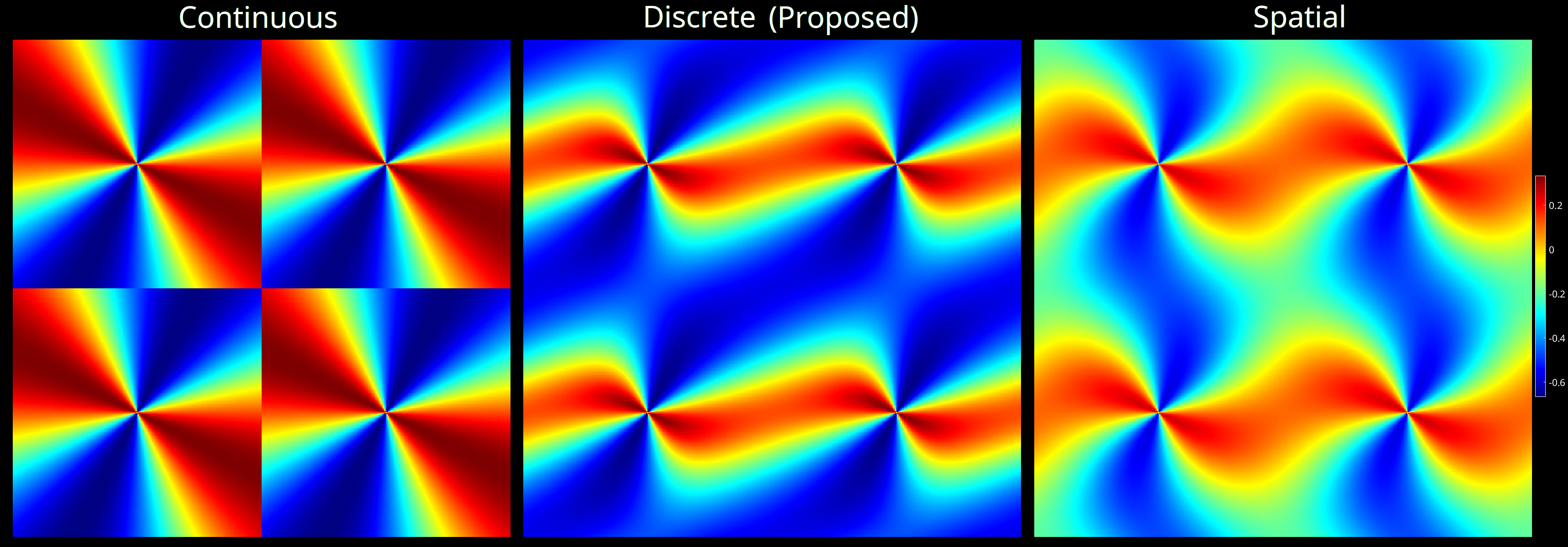
Here $$$\left\langle,\right\rangle$$$ is the complex inner product. If $$$\hat{b}_0 =[0,0,1]$$$, it is easy to show that $$$D_d$$$ corresponds to the simple discrete kernel formulation in 8. All kernels (with the FFT of the spatial kernel) and examples of striping artifacts are shown in Figure 1.
We compared the PDF results for all kernels (Continuous: Eq.2, Spatial: Eq.3, Discrete: Eq.4) in:
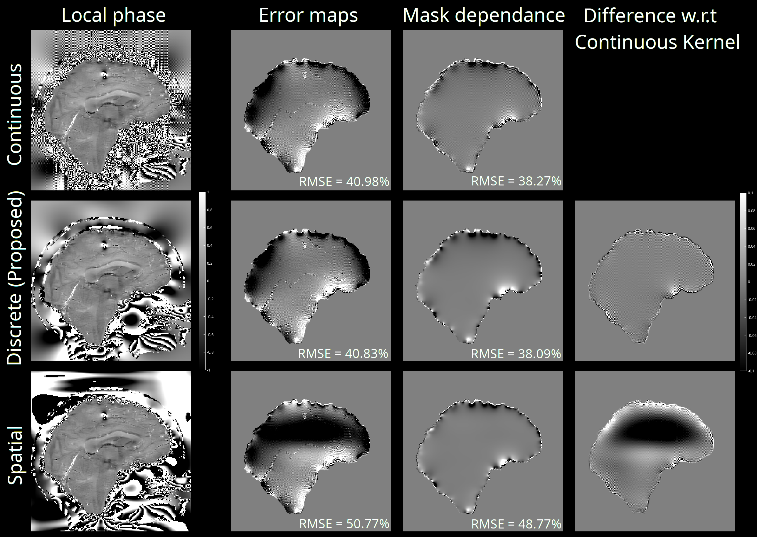
1. In silico brain phantom: Using data from the QSM Reconstruction Challenge 2.011 toolbox, we simulated the total field and assessed PDF's performance against two distinct masks. Our analysis explored the robustness of PDF against noise and boundary shape, with no angulation. The quality of solutions was evaluated using the root mean squared error (RMSE).
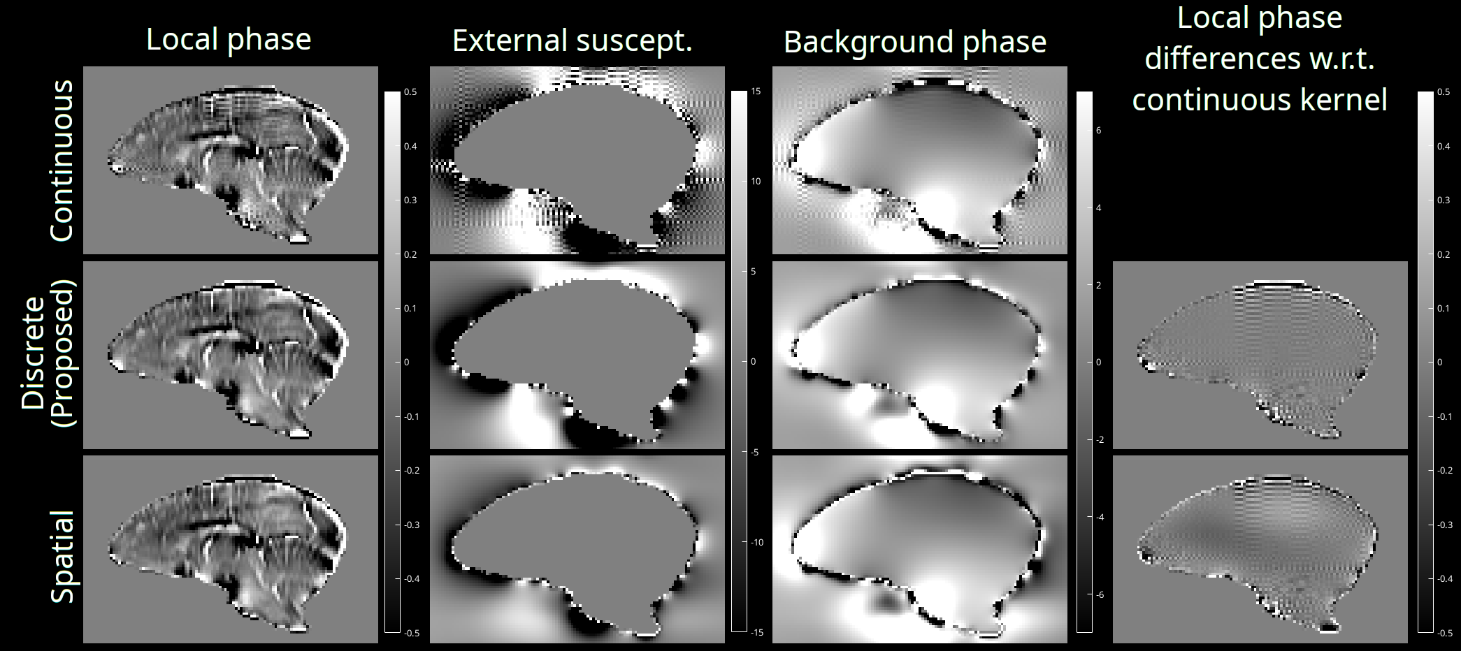
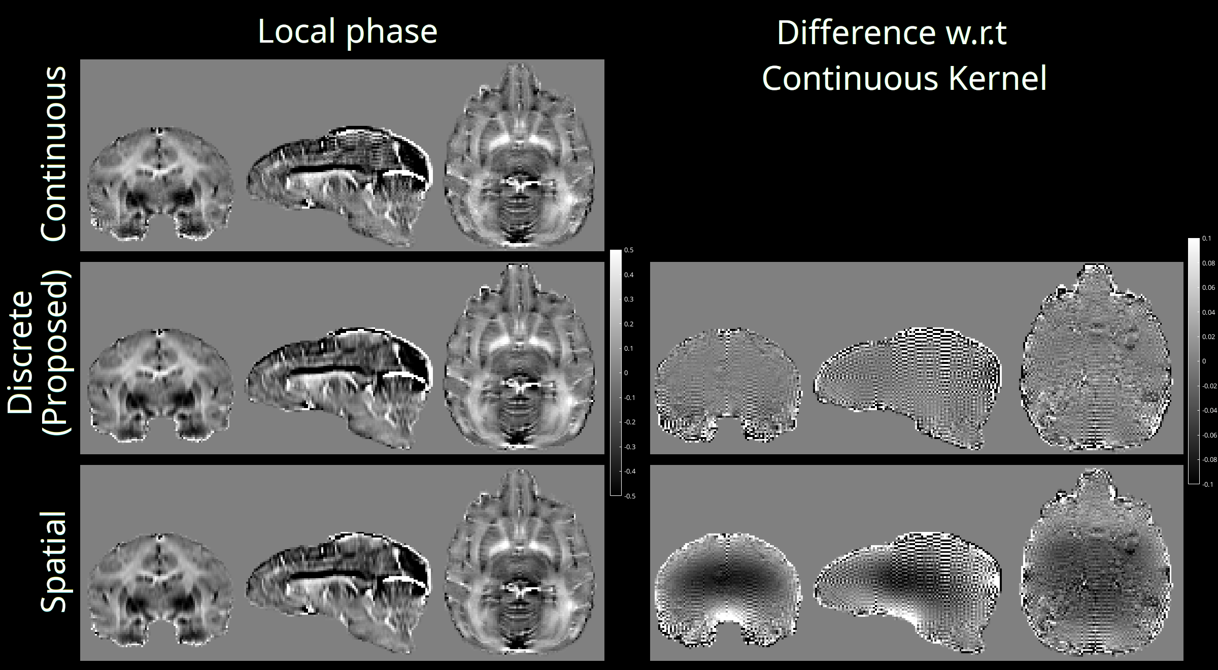
2. In vivo GRE angulated acquisitions. In this case, we evaluated the results qualitatively by inspecting the outcomes and difference maps.
The source code is available at: http://gitlab.com/cmilovic/FANSI-toolbox
RESULTS AND DISCUSSION
Our findings reveal that even when $$$B_0$$$ is aligned with the z-axis, the continuous kernel generates striping artifacts, as evident in the brain phantom experiment (Figure 2). These artifacts become more pronounced for the in vivo data with different angulations (Figures 3 and 4). In all experiments, the spatial kernel effectively reduces striping artifacts but introduces low-frequency inaccuracies. The discretization strategies appear to impact the frequency domain profile of the kernel, aligning the double cone in a spiral manner to the acquisition axis (Figure 5 shows explicitly how they avoid violation of circular continuity), although these effects are not reflected in the spatial domain (Figure 1). By overcoming the limitations of the continuous kernel, our generalized discrete method shows more accurate and reliable results.CONCLUSION
Striping artifacts at the boundaries of strong contrast sources are a crucial concern for background field calculation. Our study demonstrates that the generalized discrete kernel offers superior performance as the convolutional kernel in PDF, regardless of $$$B_0$$$ field orientation. We advocate for its use to achieve more accurate and artifact-free background field removal in MRI.Acknowledgements
CM thanks VINCI-DI Iniciacion grant from PUCV for its support. PF is supported by European Research Council Consolidator Grant DiSCo MRI SFN 770939. CT is supported by Fondecyt 1231535 and Millennium Institute for Intelligent Healthcare Engineering (ICN2021_004).References
1. Schweser F, et al. An illustrated comparison of processing methods for phase MRI and QSM: removal of background field contributions from sources outside the region of interest. NMR in Biomedicine 30.4 (2017): e3604.
2. Liu T, Khalidov I, de Rochefort L, Spincemaille P, Liu J, Tsiouris AJ, Wang Y. A novel background field removal method for MRI using projection onto dipole fields. NMR in Biomedicine. 2011 Nov;24(9):1129-36.
3. Salomir R, De Senneville BD, Moonen CTW. A fast calculation method for magnetic field inhomogeneity due to an arbitrary distribution of bulk susceptibility. Concepts Magn Reson. 2003;19B:26-34. doi:10.1002/cmr.b.10083
4. Marques J P, Bowtell R. Application of a Fourier-based method for rapid calculation of field inhomogeneity due to spatial variation of magnetic susceptibility. Concepts Magn Reson Part B Magn Reson Eng. 2005;25:65-78. doi:10.1002/cmr.b.20034
5. Kiersnowski, OC, Karsa, A, Wastling, SJ, Thornton, JS, Shmueli, K. Investigating the effect of oblique image acquisition on the accuracy of QSM and a robust tilt correction method. Magn Reson Med. 2023; 89: 1791-1808. doi:10.1002/mrm.29550
6. Dixon EC. Applications of MRI Magnetic Susceptibility Mapping in PET-MRI Brain Studies. Doctoral thesis, UCL (University College London). 2018. http://discovery.ucl.ac.uk/10053515/
7. Li L, Leigh JS. Quantifying arbitrary magnetic susceptibility distributions with MR. Magn Reson Med. 2004 May;51(5):1077-82.
8. Milovic C, Acosta-Cabronero J, Pinto JM, Mattern H, Andia M, Uribe S, Tejos C. A new discrete dipole kernel for quantitative susceptibility mapping. Magn Reson Imaging. 2018 Sep;51:7-13. doi:10.1016/j.mri.2018.04.004. Epub 2018 Apr 16. PMID: 29673893.
9. Bilgic B, Chatnuntawech I, Langkammer C, Setsompop K. Sparse Methods for Quantitative Susceptibility Mapping. Wavelets and Sparsity XVI, SPIE 2015. doi: 10.1117/12.2188535
10. Milovic C, Bilgic B, Zhao B, Acosta-Cabronero J, Tejos C. Fast nonlinear susceptibility inversion with variational regularization. Magn Reson Med. 2018;80:814-821. doi:10.1002/mrm.27073
11. Marques, JP, et al. QSM reconstruction challenge 2.0: A realistic in silico head phantom for MRI data simulation and evaluation of susceptibility mapping procedures. Magnetic resonance in medicine 86.1 (2021): 526-542.
12. Smith SM. Fast robust automated brain extraction. Hum Brain Mapp. 2002;17(3):143–155. doi: 10.1002/hbm.10062
13. QSM Consensus Organization Committee, et al. Recommended Implementation of Quantitative Susceptibility Mapping for Clinical Research in The Brain: A Consensus of the ISMRM Electro-Magnetic Tissue Properties Study Group. Preprint. 2023 Jul 5: arXiv:2307.02306v1.
Figures