0155
Spatiotemporal encoding MRI at a portable low field system without parallel imaging1School of Biomedical Engineering, Shanghai Jiao Tong University, Shanghai, China, 2National Engineering Research Center of Advanced Magnetic Resonance Technologies for Diagnosis and Therapy (NERC-AMRT), Shanghai Jiao Tong University, Shanghai, China, 3Department of Chemical and Biological Physics, Weizmann Institute of Science, Rehovot, Israel, Rehovot, Israel
Synopsis
Keywords: Low-Field MRI, Low-Field MRI, SPEN, Field Inhomogeneity, less distortion, low SAR
Motivation: Geometric distortions in echo-planar acquisitions pose challenges for correction in portable low-field MRI due to significant field inhomogeneities.
Goal(s): Our goal was to apply spatiotemporal encoding (SPEN) MRI at a 110 mT portable low-field system, aiming for nearly distortion-free echo-planar images.
Approach: We leveraged the low SAR in low-field MR to optimize the SPEN technique for substantial gains in sensitivity. SPEN-based 2D imaging ,3D imaging and DWI were compared with EPI-based imaging and EPI TopUp correction results.
Results: Approximately distortion-free SPEN acquisitions including robust 2D, 3D imaging and DWI demonstrated the potential clinical values of SPEN in the portable low field systems.
Impact: SPEN MRI provides a unique and robust fast echo planar acquisition approach to obtain nearly distortion-free images at low-cost portable low field systems, thereby expanding the prospects for rapid imaging, navigation, and functional imaging in portable low-field MRI.
Introduction
Low-field magnetic resonance imaging (MRI) offers cost-effective and portable solutions1, 2. However, while high-field superconducting magnets provide uniform B0 polarizing fields (approximately 1 ppm after passive shim), low-cost, portable magnets exhibit much less spatial homogeneity (hundreds to thousands of ppm) for head imaging3-8. This inhomogeneity poses challenges for echo-planar acquisitions due to their restricted phase-encoding bandwidth9 and limitations in parallel imaging for acceleration caused by fewer receive channels in portable MRI.Spatiotemporal encoding (SPEN) MRI has shown promise as an alternative to EPI 10, offering enhanced resistance to magnetic field inhomogeneities in a similar acquisition time 11, especially when SAR limitations are not a concern12, 13 and parallel acceleration is generally restricted in low-field MRI.
In this study, we demonstrated the capability of reducing image distortions of SPEN MRI versus the EPI counterpart at a 110 mT portable low-field system. The robustness of SPEN MRI is further evaluated with 3D imaging and diffusion-weighted MRI on human brain.
Methods
Portable 110mT MRI systemAll experiments were conducted on a prototype portable MRI system as shown in Fig.1(a). The magnet is a SmCo plate permanent magnet with field strength of 110 mT. After passive shimming, the peak-to-peak field inhomogeneity over 220 mm DSV is about 150 ppm.
SPEN sequence
By replacing the 180˚ RF pulse of SE-EPI with a frequency-swept radiofrequency chirp pulse acting in the presence of encoding Ge gradient (y axis), the SPEN sequence as shown in Fig.1(b). Remarkably, without parallel imaging or multi-shot acquisition, SPEN decreases the field inhomogeneities distortions by enlarging the blip moments, -i.e., increasing the Q value of the encoding chirp pulse. By defining a subsampling factor R = 2Q/Ny, the larger R it is, the fewer image distortions are obtained by the SPEN MRI. In the design of the frequency-swept pulse, leveraging the low SAR value in the low-field setting allowed us to reduce its duration time to 4 ms.
In vivo experiments
For the 2D SPEN and EPI: TR/TE = 10000/105 ms; echo spacing = 0.98 ms; NEX = 6; acquisition matrix size = 96 × 96; slice thickness = 10mm; resolution =2.5 × 2.5 mm2. For the 3D SPEN and EPI: TR/TE = 2000/105 ms; echo spacing = 0.98 ms; NEX = 1; acquisition matrix size = 96 × 96 × 96; resolution =2.5 × 2.5 × 2.5 mm3. For the SPEN and EPI DWI: TR/TE = 5000/125 m; echo spacing = 0.82 ms; NEX = 18; acquisition matrix size =80 × 80; slice thickness = 10mm; resolution =3 × 3 mm2. For all experiments, acquisition bandwidth = 100kHz.
Results
Figure 2 displays a comparison between 2D EPI and SPEN under identical sampling conditions. The distortions in EPI image correspond to the B0 map, and the distortion resistance of SPEN improves with increasing R. Figure 3 displays the comparison between EPI images corrected using TopUp and SPEN images (R = 2) with different numbers of averages. When fewer averages are applied, TopUp-corrected images exhibit lower SNR, and structures within the dashed yellow boxes in the TopUp images are notably blurred. Figure 4 provides a comparison between 3D EPI and 3D SPEN(R=2). Figure 5 illustrates the SPEN DWI (R=2) and EPI DWI images.Disscusion and Conclusions
For the adiabatic pulse, reducing its duration (Tp in Fig.1) time increases the power, especially when a large Q is applied. As SAR is proportional to the square of the field strength, we can achieve shorter Tp than those possible at high fields. Although Tp<Ta/2 (see in Figure 1) theoretically leads to T2* contrast weighting14, the obtained SPEN images at low fields exhibit similar contrast to the EPI images. Shortening the duration of the adiabatic pulse provides several advantages, including creating more time for the acquisition echo, improving SNR, and enabling better contrast design. This is crucial for DWI, as limited gradient performance leads to longer diffusion gradient durations.TopUp imposes specific demands on image SNR and the stability of scans in two PE directions. However, the instability of portable low-field MRI systems and motion artifacts induced during prolonged averaging negatively impact TopUp results (see Fig. 3). In contrast, SPEN sequences, needing just one scan, alleviate these concerns.
SPEN MRI provides a robust fast echo planar acquisition approach to obtain less distorted images or even distortion-free images at low-cost portable low-field systems
Acknowledgements
This work is supported by the National Natural Science Foundation of China National Science Foundation of China (No. 62001290 and 62301309), Shanghai Science and Technology Development Funds (21DZ1100300) and sponsored by the National Science and Technology Innovation 2030 Major Project (2022ZD0208601).References
1. Campbell-Washburn, A.E., et al., Opportunities in Interventional and Diagnostic Imaging by Using High-Performance Low-Field-Strength MRI. Radiology, 2019. 293(2): p. 384-393.
2. Marques, J.P., et al., ESMRMB annual meeting roundtable discussion:“when less is more: the view of MRI vendors on low-field MRI”. Magnetic Resonance Materials in Physics, Biology and Medicine, 2021. 34(4): p. 479-482.
3. Gach, H.M., et al., B(0) field homogeneity recommendations, specifications, and measurement units for MRI in radiation therapy. Med Phys, 2020. 47(9): p. 4101-4114.
4. Liu, Y., et al., A low-cost and shielding-free ultra-low-field brain MRI scanner. Nature communications, 2021. 12(1): p. 1-14.
5. Marques, J.P., F.F.J. Simonis, and A.G. Webb, Low-field MRI: An MR physics perspective. J Magn Reson Imaging, 2019. 49(6): p. 1528-1542.
6. Sarracanie, M. and N. Salameh, Low-Field MRI: How Low Can We Go? A Fresh View on an Old Debate. Frontiers in Physics, 2020. 8.
7. Tayler, M.C. and D. Sakellariou, Low-cost, pseudo-Halbach dipole magnets for NMR. Journal of Magnetic Resonance, 2017. 277: p. 143-148.
8. O’Reilly, T., et al., In vivo 3D brain and extremity MRI at 50 mT using a permanent magnet Halbach array. Magnetic Resonance in Medicine, 2020. 85(1): p. 495-505.
9. Morgan, P.S., et al., Correction of spatial distortion in EPI due to inhomogeneous static magnetic fields using the reversed gradient method. Journal of Magnetic Resonance Imaging, 2004. 19(4): p. 499-507.
10. Shrot, Y. and L. Frydman, Spatially encoded NMR and the acquisition of 2D magnetic resonance images within a single scan. Journal of Magnetic Resonance, 2005. 172(2): p. 179-190.
11. Ben-Eliezer, N., Y. Shrot, and L. Frydman, High-definition, single-scan 2D MRI in inhomogeneous fields using spatial encoding methods. Magnetic resonance imaging, 2010. 28(1): p. 77-86.
12. Runge, V.M. and J.T. Heverhagen, The Clinical Utility of Magnetic Resonance Imaging According to Field Strength, Specifically Addressing the Breadth of Current State-of-the-Art Systems, Which Include 0.55 T, 1.5 T, 3 T, and 7 T. Invest Radiol, 2022. 57(1): p. 1-12.
13. Wujciak, D., Modern mid-field magnetic resonance imaging in private practice: Field report. Der Radiologe, 2022. 62(5): p. 405-409.
14. Ben-Eliezer, N., et al., Fully refocused multi-shot spatiotemporally encoded MRI: robust imaging in the presence of metallic implants. Magnetic Resonance Materials in Physics, Biology and Medicine, 2012. 25: p. 433-442.
Figures
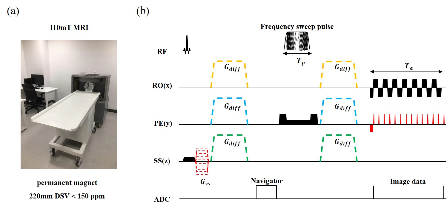
FIGURE 1. SPEN sequences with the options of diffusion weighted imaging or 3D acquisition. (a) The prototype 110mT portable MRI system employed in this study.(b)The duration of the 180° swept refocusing pulse in the figure is denoted as Tp. The duration of the acquisition window is denoted as Ta. Gss represents the phase encoding in the slice direction used in 3D SPEN, while Gdiff is the diffusion gradient module employed in SPEN DWI experiments.
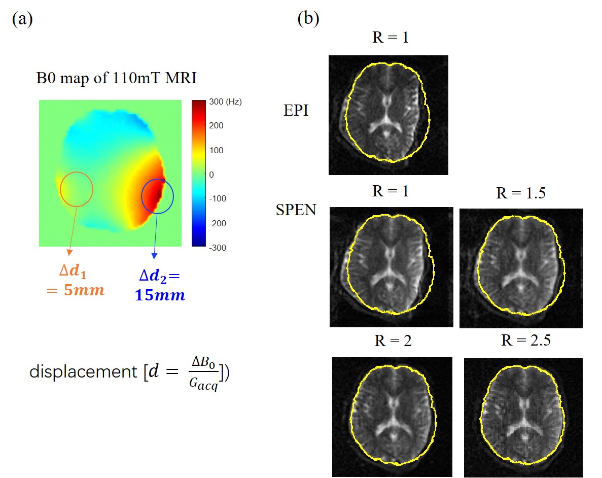
FIGURE 2. 2D EPI vs SPEN results. (a) The figure depicts a 2D B0 map of the human brain obtained during the experiment. The B0 map allows us to estimate image distortion using theoretical formulas. In (b) a comparison is made between 2D EPI and SPEN images. The first row displays EPI images, while the following two rows present SPEN images at subsampling rates of R=1, 1.5, 2, and 2.5. The yellow border marks the brain boundary extracted under the SE sequence. It is evident that as the subsampling rate increases, SPEN images exhibit reduced distortion.
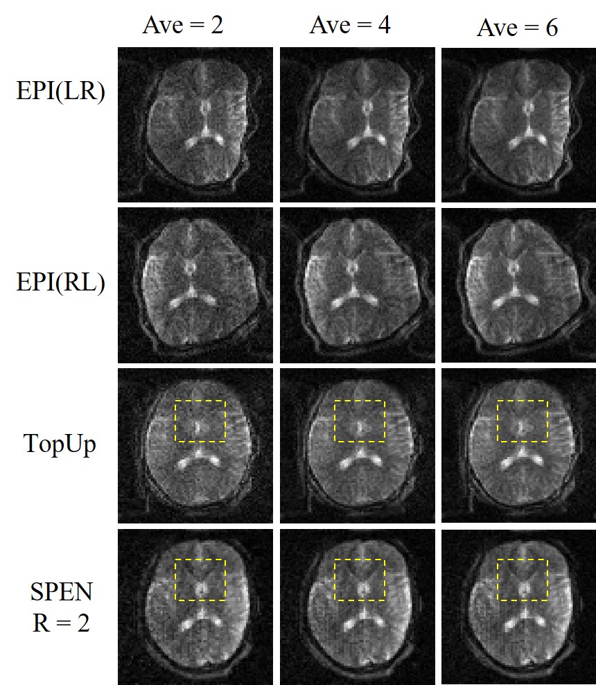
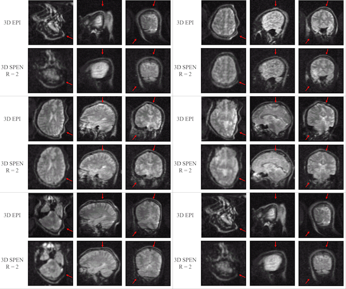
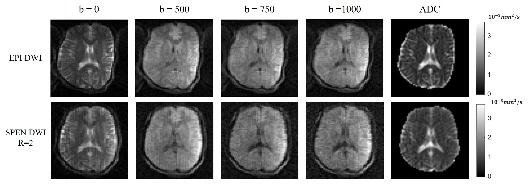
FIGURE 5. DWI SPEN vs DWI EPI results. The first row displays the EPI DWI results, while the second row presents the SPEN DWI results. The first four columns show the DWI results for b=0 s/mm2, b=500 s/mm2, b=750 s/mm2, and b=1000 s/mm2, respectively. The last column exhibits the ADC image. It is evident that the distortion in SPEN DWI images is significantly reduced compared to EPI DWI images.