0118

Blind spherical deconvolution of multi-shell diffusion MRI to model regional changes in pathology

Siebe Leysen^1,2, Ahmed Radwan^2,3, Frederik Maes^1,2, Stefan Sunaert^2,3,4, and Daan Christiaens^1,2,3
¹Department of Electrical Engineering, ESAT/PSI, KU Leuven, Leuven, Belgium, ²Medical Imaging Research Center, UZ Leuven, Leuven, Belgium, ³Department of Imaging and Pathology, Translational MRI, KU Leuven, Leuven, Belgium, ⁴Department of Radiology, KU Leuven, Leuven, Belgium

Synopsis

Keywords: Diffusion Modeling, Signal Representations

Motivation: Diffusion-weighted MRI (dMRI) has significantly enhanced our ability to investigate the brain's microstructure, but analysis in pathology remains difficult.

Goal(s): This study introduces a voxelwise approach to concurrently estimate the Orientation Distribution Function (ODF) and response function for fiber orientation analysis and tractography.

Approach: The proposed blind deconvolution method models the kernel as a sum of axially-symmetric Gaussian functions, defined in spherical harmonics. It is evaluated through simulations and in-vivo experiments in healthy volunteers and glioma patients, demonstrating its efficacy in ODF estimation and data fitting.

Results: This novel approach presents better modeling of pathology and offers promising results for white matter analysis.

Impact: We introduce a blind deconvolution method for brain microstructure analysis with DWI that concurrently estimates a voxelwise ODF and kernel. This method can aid tractography and provide new image contrasts in the presence of pathology.

Introduction

Diffusion-weighted MRI (dMRI) has revolutionized our ability to non-invasively explore brain tissue microstructure and connectivity^1,2. Among various techniques, multi-tissue constrained spherical convolution (MT-CSD)³ is widely used to estimate the fiber orientation distribution function (ODF) used in tractography. However, MT-CSD relies on tissue-specific response functions, estimated globally for predetermined tissue types such as white and gray matter, which can be hard to define in lesions and other structural pathology. To overcome these limitations, we aim to concurrently estimate local response functions and ODFs, with minimal prior assumptions on the underlying tissue microstructure. The voxel-wise response function is well-suited to model data with unknown tissue types and pathology.

Method

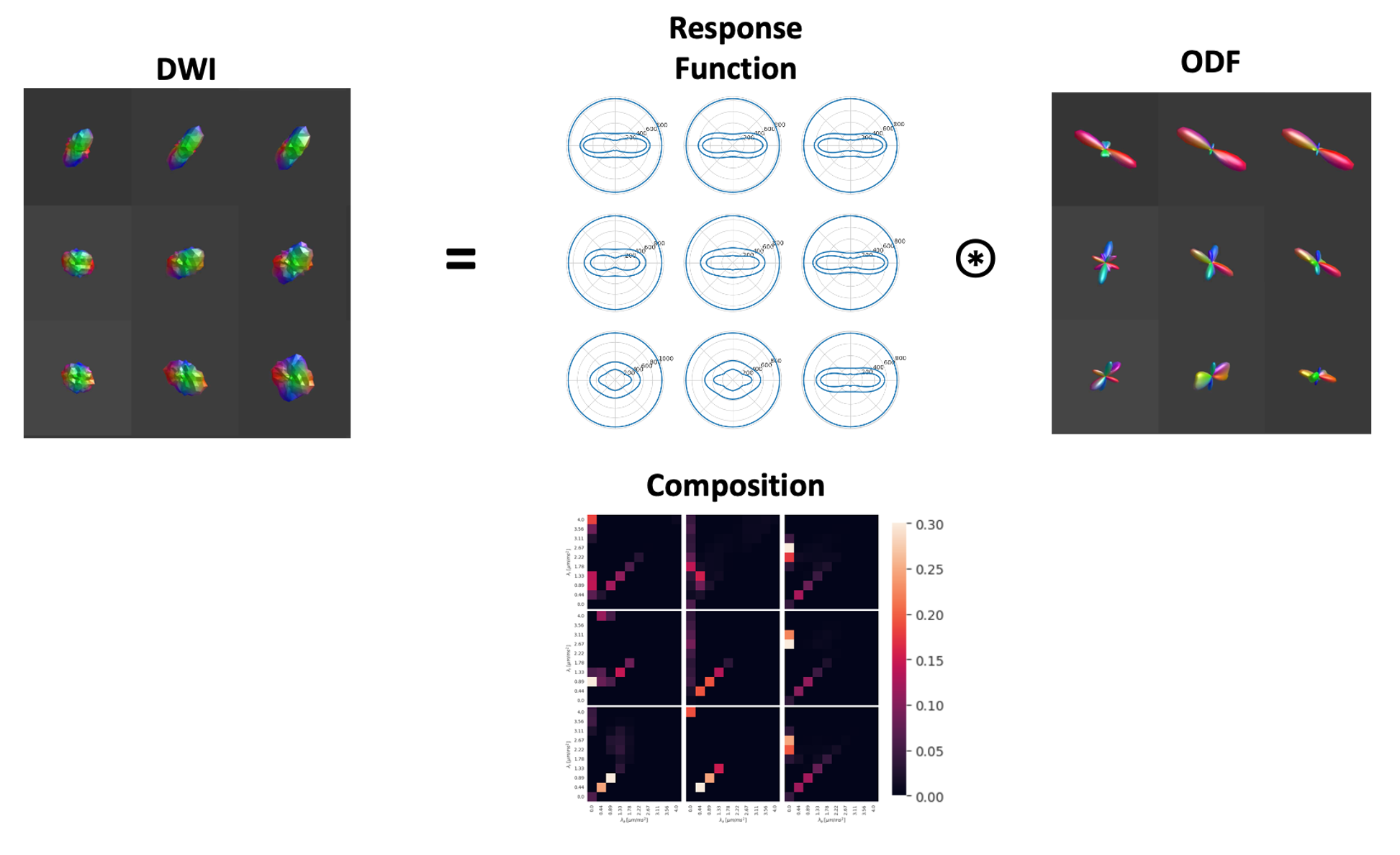
Blind Deconvolution The signal $$$S$$$ in each voxel is modeled as a single spherical convolution of a voxelwise response function $$$H$$$ and an ODF $$$P$$$⁴ (Fig.1). We represent the response function $$$H$$$ as a weighted sum of axially-symmetric Gaussian functions $$$G(\lambda_a,\lambda_ r)$$$ represented in zonal spherical harmonics. The Gaussian functions are defined on a discrete grid of axial ($$$\lambda_a$$$ ) and radial ($$$\lambda_r$$$) diffusivities, defined as 10 linearly spaced values in the range$$$ [0, 4] \mu m^2/ms$$$ with $$$\lambda_r\leq\lambda_a$$$ . The response function hence represents a linear mixture model of microstructural compartments in a fully data-driven way. The objective is to jointly estimate the mixture fractions $$$f_{a,r}$$$ that represent the response and the SH coefficients that represent the ODF.
The resulting blind spherical deconvolution is ill-conditioned, i.e., infinitely many solutions exist that accurately represent the signal. To cope with this, we 1) unit-normalize the ODF, 2) constrain ODF nonnegativity, and 3) introduce regularization on the response function smoothness, defined as the squared norm of all SH components with SH order ℓ> 0. This regularization promotes more spherically-shaped response functions, which in turn encourages ODF sparsity. Regularization weight $$$\lambda=10^{-4}$$$ was found to be a sensible trade-off, irrespective of the dataset.
$$\begin{equation*}\boxed{\begin{aligned}\min_{P, H}\quad & \sum_{\ell\in\{0, 2,…,\ell_{max}\}}{\left(S_\ell-\mathscr{N}_\ell H_\ell P_\ell^\top\right)}^2+\lambda\sum_{b,\ell>0}H^2_{b,\ell}\\ \textrm{s.t.}\quad & QP^\top \geq 0\\&H=S_0\sum_{\lambda_a=0}^{\lambda_a^{(max)}}\sum_{\lambda_r=\lambda_a}^{\lambda_r^{(max)}}f_{a,r}G(\lambda_a,\lambda_r)\;\;\;\;\;0\leq f_{a, r}\leq1\\ &\sum_{a=0}^{\lambda_a^{(max)}} \sum_{r = a}^{\lambda_r^{(max)}}f_{a,r}=1\end{aligned}}\end{equation*}$$
Experimental Design The proposed method is validated in simulations using dMRI encoding that comprises b=0,1000,2000 $$$s/mm^2$$$ (2,128,128 directions). Data is generated by forward spherical convolution of predefined ODF (single fiber and 60°-crossing) and response function pairs. The simulated response function comprises stick, zeppelin and free water compartments, accounting for 45%, 45% and 10% respectively. The simulation is repeated 500 times using different Rician noise realizations.
Data In-vivo data from one healthy volunteer (encoding identical to simulation) and 11 low- and high-grade glioma datasets (5 b=0 $$$s/mm^2$$$, 128 b=1200 $$$s/mm^2$$$ and 125 b=2500 $$$s/mm^2$$$) are examined. All data is acquired on a 3T Philips Achieva MRI with a 32-channel dStream head coil at 2mm isotropic resolution. SNR levels in white matter are estimated at acquisition time.

Results

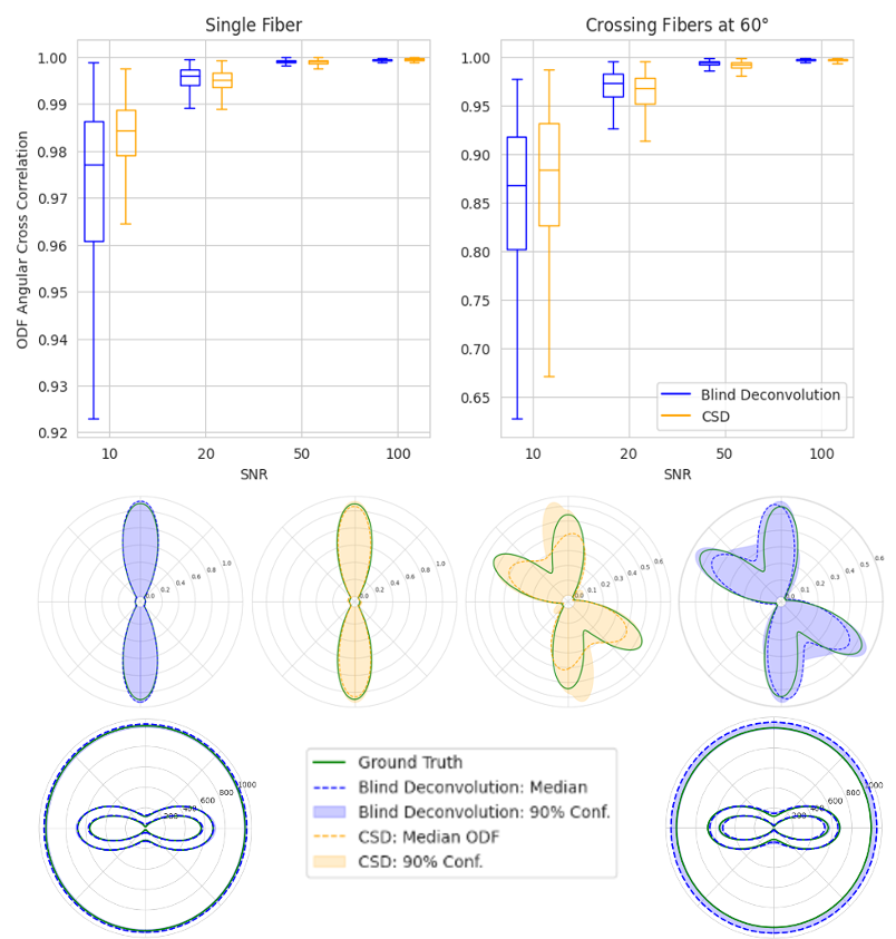
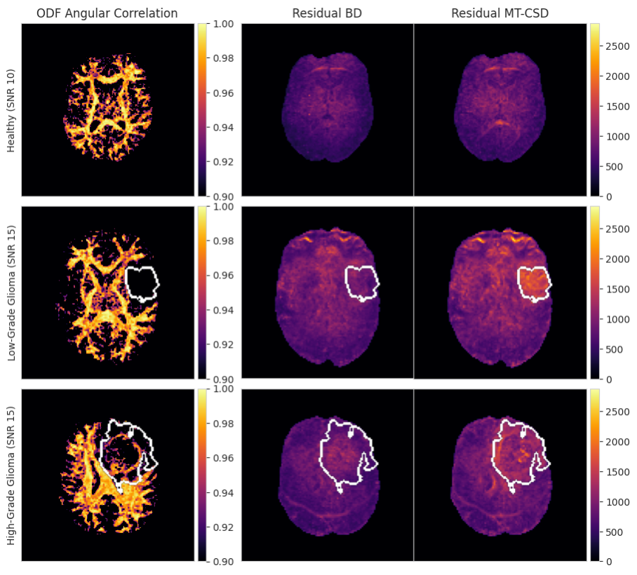
Figure 2 presents boxplots of the angular cross-correlation⁵ between the ODF estimation of the proposed method and MSMT-CSD as well as a visualization of the 90% confidence interval of the estimated crossing fiber ODFs and response functions at SNR 20.
Figure 3 shows the angular cross-correlation and signal residual maps for three in vivo datasets: healthy adult brain, low-grade glioma and high-grade glioma.
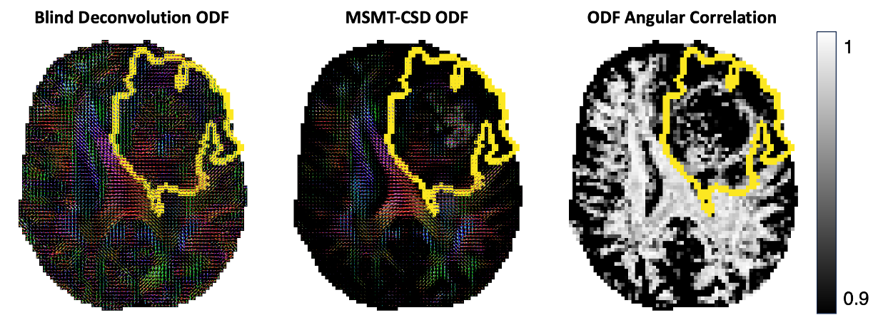
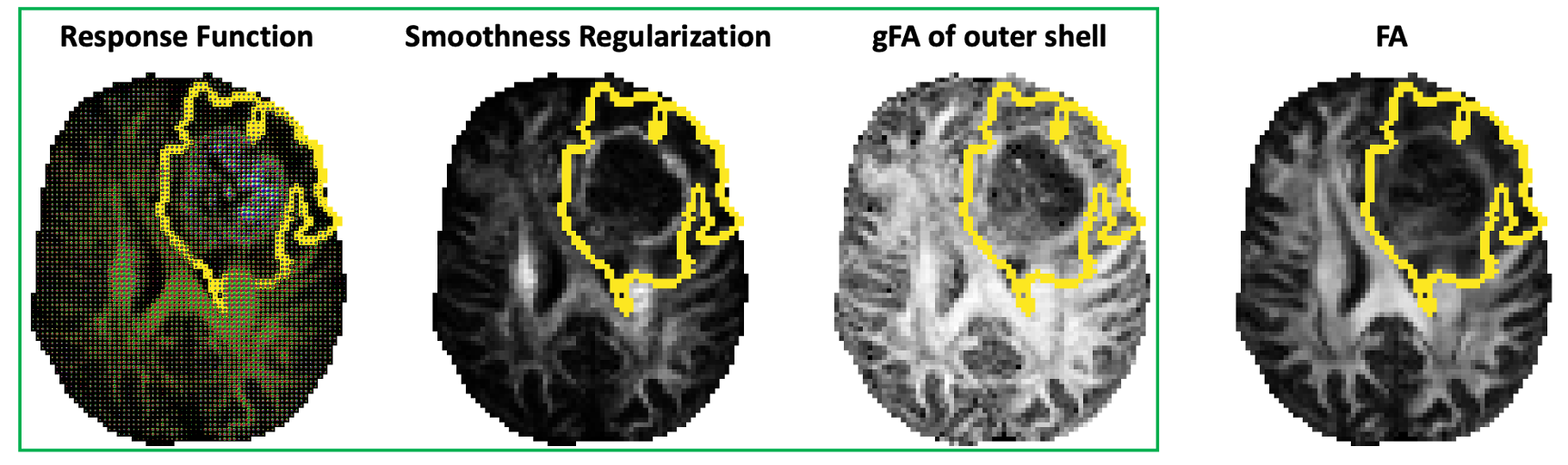
Visualizations of ODF estimations by MSMT-CSD and Blind Deconvolution are shown in Figure 4. Figure 5 shows the estimated response functions, the regularization term as a contrast and the generalized fractional anisotropy (gFA) of these response functions⁶.

Discussion

At SNR$$$\geq$$$20, the performance of blind deconvolution in simulations is on par with CSD, despite the latter using the ground truth response function. Figure 2 shows that both ODF and response function estimation are close to the ground truth at SNR 20 with ODF deviations similar to the errors in CSD.
In in vivo data, blind deconvolution provides ODF estimates which align closely to CSD while providing better data fit as can be seen by the lower residuals in Figure 3. This difference in residual is more significant in the presence of pathology, indicating that not assuming a canonical kernel has a significant impact.

Conclusion

We modeled dMRI data through a voxelwise blind spherical deconvolution, and demonstrated more accurate representation of pathological data. In contrast to prior work estimating per-voxel response functions^5,7, we model the response function as a mixture of Gaussians which allows us to model multiple microstructural compartments. The estimated voxelwise response functions provide new image contrasts such as kernel-GFA shown in Fig. 5 to study tissue microstructure in pathology.

Acknowledgements

This work is supported in part by the Internal Funds KU Leuven under Grant C24/18/047 and by the Flemish Government under the “Onderzoeksprogramma Artificiële Intelligentie (AI) Vlaanderen” programme.

References

¹le Bihan, D., Mangin, J. F., Poupon, C., Clark, C. A., Pappata, S., Molko, N., & Chabriat, H. (2001). Diffusion tensor imaging: concepts and applications. Journal of Magnetic Resonance Imaging : JMRI, 13(4), 534–546. https://doi.org/10.1002/JMRI.1076

²Jones, PhD, Derek K. (ed.), Diffusion MRI: Theory, Methods, and Applications (2010; online edn, Oxford Academic, 1 Sept. 2012), https://doi.org/10.1093/med/9780195369779.001.0001, accessed 4 Nov. 2023.

³Jeurissen, B., Tournier, J. D., Dhollander, T., Connelly, A., & Sijbers, J. (2014). Multi-tissue constrained spherical deconvolution for improved analysis of multi-shell diffusion MRI data. NeuroImage, 103, 411–426. https://doi.org/10.1016/J.NEUROIMAGE.2014.07.061

⁴Christiaens, D., Veraart, J., Cordero-Grande, L., Price, A. N., Hutter, J., Hajnal, J. v., & Tournier, J. D. (2020). On the need for bundle-specific microstructure kernels in diffusion MRI. NeuroImage, 208, 116460. https://doi.org/10.1016/J.NEUROIMAGE.2019.116460

⁵Anderson, A. W. (2005). Measurement of fiber orientation distributions using high angular resolution diffusion imaging. Magnetic Resonance in Medicine, 54(5), 1194–1206. https://doi.org/10.1002/MRM.20667

⁶Glenn, G. R., Helpern, J. A., Tabesh, A., & Jensen, J. H. (2015). Quantitative Assessment of Diffusional Kurtosis Anisotropy. NMR in Biomedicine, 28(4), 448. https://doi.org/10.1002/NBM.3271

⁷Schultz, T., & Groeschel, S. (2013). Auto-calibrating spherical deconvolution based on ODF sparsity. Lecture Notes in Computer Science (Including Subseries Lecture Notes in Artificial Intelligence and Lecture Notes in Bioinformatics), 8149 LNCS(PART 1), 663–670. https://doi.org/10.1007/978-3-642-40811-3_83/COVER

Figures

Visual representation of the proposed method in 9 voxels at the GM-WM-interface. The signal is represented as the spherical deconvolution of per-voxel response functions and ODFs. The response function is modeled as the weighted sum of axially-symmetric Gaussian functions, shown in the bottom plot.

Boxplots of the angular correlation between blind deconvolution and the ground truth show close alignment with CSD. 90% confidence intervals of the ODF and response function are plotted below the box plots. The response function is only shown for blind deconvolution, CSD uses the ground truth response function.

Angular correlation maps between Blind Deconvolution and MT-CSD show close correspondence in white matter. Blind Deconvolution consistently produces lower residual maps than MT-CSD, especially in tumor regions delineated in white. The mentioned SNR values are estimated at acquisition time.

Axial slice of ODF estimations by blind deconvolution and MT-CSD. The right plot shows the angular correlation between both estimations. Angular correlation in healthy white matter is close to 1. The scale difference in the ODF estimations are caused by the ODF being unit-normalized in blind deconvolution. In MT-CSD the ODF size is related to white matter volume fraction.

Axial slice of response function estimation using blind deconvolution. The green bounding box represents the estimation of the response function and two derived contrasts. Both of these contrasts exhibit similarities with the fractional anisotropy map, which is to be expected. The smoothness term in the objective function and gFA are both based on kernel anisotropy.

Proc. Intl. Soc. Mag. Reson. Med. 32 (2024)

0118

DOI: https://doi.org/10.58530/2024/0118