0046
Image recovery using deep end-to-end posterior networks1University of Iowa, Iowa city, IA, United States
Synopsis
Keywords: Image Reconstruction, Data Processing
Motivation: End-to-End (E2E) trained unrolled algorithms recover MR images with high quality. However, they have large memory demands during training. In addition, these maximum a posteriori methods cannot provide uncertainty estimates.
Goal(s): To develop a memory-efficient framework for E2E learning of the posterior probability distribution.
Approach: We model the posterior distribution as a combination of the data-consistent-determined likelihood term and the prior, represented using a Convolutional Neural Network whose weights are learned in an E2E fashion using maximum likelihood optimization.
Results: The proposed E2E training strategy requires significantly less memory than unrolling. In addition, the model facilitates sampling and provides uncertainty estimates.
Impact: The higher memory efficiency of the proposed E2E scheme makes it an attractive option for image reconstruction problems of large dimensions. The learned posterior model provides a minimum mean square estimate and uncertainty maps, which unrolled approaches cannot offer.
Introduction
Unrolled algorithms[1,2] that utilize End-to-End (E2E) trained Convolutional Neural Networks (CNN) offer state-of-the-art reconstruction performance. However, their training is memory intensive, which hinders their use in high dimensional applications. To reduce the memory demand, Deep Equilibrium Models[3,4] (DEQ) were introduced, which require the CNN to be a contraction that restricts the reconstruction performance. Moreover, unrolled and DEQ algorithms cannot provide uncertainty maps. While diffusion approaches[5] can offer Minimum Mean Square Error (MMSE) estimates and uncertainty maps, they do not rely on E2E optimization and require numerous iterations during inference.We introduce a memory-efficient Deep E2E Posterior Network (DEEPEN) to tackle the above challenges. Unlike current E2E models that learn the Maximum A Posteriori (MAP) estimate, we learn the posterior distribution. We model the posterior as the sum of a likelihood term and a CNN prior. The CNN parameters are E2E learned using Maximum Likelihood (ML), which eliminates algorithm unrolling and Lipschitz constraint. The learned model can be used to derive the MAP estimate, and the posterior can be sampled to obtain an MMSE estimate and uncertainty maps.
Methods
We consider the recovery of MR image $$$\mathbf{x}\in\mathbb{C}^m$$$ from its corrupted undersampled measurements $$$\mathbf{b}\in\mathbb{C}^n$$$:$$\begin{equation}\mathbf{b}=\mathbf{A}\mathbf{x}+\mathbf{n}\end{equation}\hspace{20mm}(1)$$
where $$$\mathbf{A}\in\mathbb{C}^{n \times m}$$$ is known and $$$\mathbf{n}\in\mathcal{N}(0,\eta^2\mathbf{I})$$$. Given the measurements, we model the negative log posterior of the image as:
$$\begin{equation}-\log p_\boldsymbol\theta(\mathbf{x}|\mathbf{b})= \underbrace{\dfrac{\|\mathbf{A}\mathbf{x}-\mathbf{b}\|^{2}}{2\eta^2}+P}_{-\log p(\mathbf{b}|\mathbf{x})} -\log p_\boldsymbol \theta (\mathbf{x})\end{equation}\hspace{20mm}(2)$$
where $$$p(\mathbf{b}|\mathbf{x})$$$ is the likelihood of observing the measurements given the MR image, $$$p_\boldsymbol\theta(\mathbf{x})$$$ models the prior $$$p(\mathbf{x})$$$ of the MR image as an Energy Based Model[6](EBM):$$p_\boldsymbol\theta(\mathbf{x})=\dfrac{1}{Z_{\boldsymbol\theta}}\exp(-E_{\boldsymbol\theta}(\mathbf{x}))\hspace{20mm}(3)$$
where the energy $$$E_{\boldsymbol\theta}(\mathbf{x}):\mathbb{C}^m\rightarrow\mathbb{R}^+$$$ is a neural network with $$$\boldsymbol\theta$$$ denoting its parameters, and $$$Z_{\boldsymbol\theta}$$$ is the normalization constant. We illustrate the energy model in Fig. 1.
ML training of the Posterior:
The optimal weights of the energy $$$E_{\boldsymbol\theta}(\mathbf{x})$$$ is determined by minimizing the negative log-likelihood of the training dataset:
$$\begin{eqnarray}\boldsymbol\theta^*&=&\arg\min_{\boldsymbol\theta}\:\mathbb{E}_{\mathbf{x}\sim q(\mathbf{x})}\Big[\underbrace{-\log p_{\boldsymbol\theta}(\mathbf{x}|\mathbf{b})}_{\mathcal L_{\boldsymbol\theta}(\mathbf{x})}\Big]\end{eqnarray}\hspace{20mm}(4)$$where $$$q(\mathbf{x})$$$ is the probability distribution of the data. Using algebraic manipulations, the gradient of the cost function in (4) can be written as:
$$\begin{eqnarray}\nabla_{\boldsymbol\theta}\mathcal{L}_{\boldsymbol\theta}(\boldsymbol{x})= \mathbb{E}_{\mathbf{x} \sim q(\mathbf{x})} [\nabla_{\boldsymbol \theta} E_{\boldsymbol\theta}(\mathbf{x})] - \mathbb{E}_{\mathbf{x} \sim p_{\boldsymbol \theta}(\mathbf{x}|\mathbf{b})}[\nabla_{\boldsymbol \theta} E_{\boldsymbol\theta}(\mathbf{x})] \end{eqnarray}\approx \left(\dfrac{1}{n} \displaystyle \sum_{i=1}^{n}{\nabla_{\boldsymbol \theta}E_{\boldsymbol \theta}(\mathbf{x}^{+}_i)}-\dfrac{1}{m}\displaystyle \sum_{j=1}^{m}{\nabla_{\boldsymbol \theta}E_{\boldsymbol \theta}(\mathbf{x}^{-}_j)}\right)\hspace{20mm}(5)$$
where $$$\mathbf{x} \sim p_{\boldsymbol \theta}(\mathbf{x}|\mathbf{b})$$$ are samples from the learned posterior distribution $$$p_{\boldsymbol \theta}(\mathbf{x}|\mathbf{b})$$$. In the EBM literature, these are the generated or fake samples denoted by $$$\mathbf{x}^-$$$, while the training samples are referred to as true samples, denoted by $$$\mathbf{x}^+ \sim q(\mathbf{x})$$$. Thus the training strategy (5) will seek to decrease $$$E_\boldsymbol{\theta}(\mathbf{x}^+)$$$, increase $$$E_\boldsymbol{\theta}(\mathbf{x}^-)$$$, and converge when $$$E_\boldsymbol{\theta}(\mathbf{x}^+)\approx E_\boldsymbol{\theta}(\mathbf{x}^-).$$$
Fake sample generation via Markov chain Monte Carlo (MCMC):
The fake samples are generated using Langevin MCMC method:
$$\begin{equation}\begin{array}{ll}\mathbf{x}_{n+1}=\mathbf{x}_n - \dfrac{\epsilon^2}{2} \left(\mathbf{A}^H(\mathbf{A}\mathbf{x}_n-\mathbf{b})+\nabla_\mathbf{x} E_{\boldsymbol \theta}(\mathbf{x}_n)\right)+ \epsilon\mathbf{z}_n \end{array}\end{equation}\hspace{20mm}(6)$$
where $$$\epsilon>0$$$ is the step-size and $$$\mathbf{z}_n \sim \mathcal{N}(0,\mathbf{I})$$$. We summarize the training process in Fig. 2.
MAP image recovery and uncertainty estimates:
Once the posterior parameters are learned, the MAP estimate is obtained by minimizing the negative log posterior distribution (2) w.r.t. $$$\mathbf{x}$$$ using the gradient descent algorithm:
$$\begin{equation}\mathbf{x}_{k+1} = \mathbf{x}_k - \alpha_k \left(\mathbf{A}^H(\mathbf{A}\mathbf{x}_k-\mathbf{b})+\nabla_x E_{\boldsymbol\theta}(\mathbf{x}_k)\right)\end{equation}\hspace{20mm}(7)$$
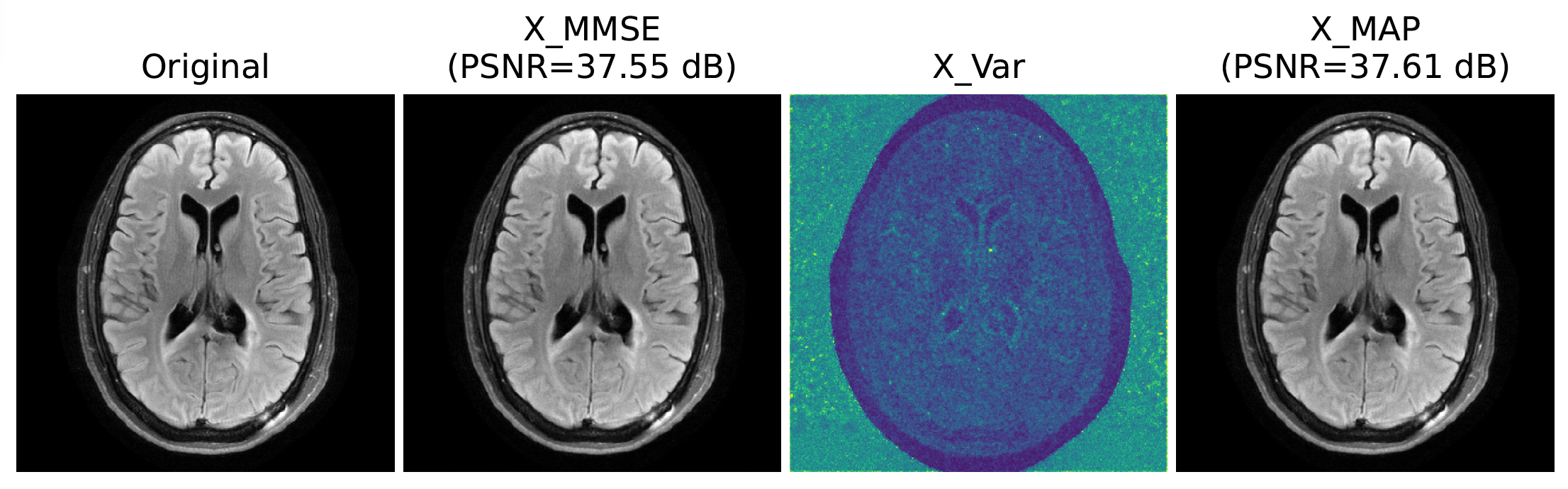
where $$$\alpha_k$$$ denotes the step-size and can be found using backtracking line search. An advantage of learning the posterior distribution is that the MMSE and the uncertainty maps about the reconstruction can be estimated by computing the mean and variance of a large number of samples from the posterior distribution. The samples are drawn using (6).
Results
We compare DEEPEN MAP estimates with MoDL[1], MoL[4], and SENSE[7] on FLAIR and T2-weighted images in the FastMRI[8] brain dataset. All E2E models were trained and evaluated on both contrasts separately for four-fold acceleration using a 1D nonuniform variable density mask. The reconstruction results are shown in Fig. 3. From the figure, we observe that DEEPEN performs better than MoL, whose lower performance is because of the Lipschitz constraint on the CNN. DEEPEN and MoDL exhibit similar performance; the significantly lower memory requirements of DEEPEN can be harnessed to reconstruct images of higher dimensions.We demonstrate the utility of DEEPEN to estimate the MMSE and the uncertainty maps in Fig. 4. The MMSE and the uncertainty maps were estimated by computing the mean and variance of $$$100$$$ samples from the posterior distribution, each sample obtained through $$$30$$$ iterations of (6) with $$$\mathbf{x}_{0}$$$ drawn randomly from a Gaussian distribution.
Conclusion
We proposed DEEPEN, a memory-efficient E2E framework that does not require unrolling and eliminates constraining the Lipschitz constant of the CNN. DEEPEN learns the posterior distribution which enables generating data consistent images.Acknowledgements
This work is supported by NIH grants R01-AG067078, R01-EB031169, and R01-EB019961.References
1. H. K. Aggarwal, M. P. Mani, and M. Jacob, “Modl: Model-based deep learning architecture for inverse problems,” IEEE transactions on medical imaging, vol. 38, no. 2, pp. 394–405, 2018.
2. K. Hammernik et al., "Learning a variational network for reconstruction of accelerated MRI data," Magnetic Resonance in Medicine, vol.79, no. 6, pp. 3055--3071, 2018.
3. S. Bai, J. Z. Kolter, and V. Koltun, “Deep equilibrium models,” Advances in Neural Information Processing Systems, vol. 32, 2019.
4. A. Pramanik, M. B. Zimmerman, and M. Jacob, “Memory-efficient model-based deep learning with convergence and robustness guarantees,” IEEE Transactions on Computational Imaging, vol. 9, pp. 260–275, 2023.
5. G. Luo, M. Blumenthal, M. Heide et al., “Bayesian MRI reconstruction with joint uncertainty estimation using diffusion models,” Magnetic Resonance in Medicine, vol. 90, no.1, pp.295-311, 2023.
6. Song and D. P. Kingma, “How to train your energy-based models,” arXiv preprint arXiv:2101.03288, 2021.
7. P. Pruessmann et al., “Sense: sensitivity encoding for fast mri,”Magnetic Resonance in Medicine: An Official Journal of the International Society for Magnetic Resonance in Medicine, vol. 42, no. 5, pp. 952–962, 1999.
8. J. Zbontar, F. Knoll, A. Sriram et al., “Fastmri: An open dataset and benchmarks for accelerated MRI,” arXiv preprint arXiv:1811.08839, 2018.
Figures
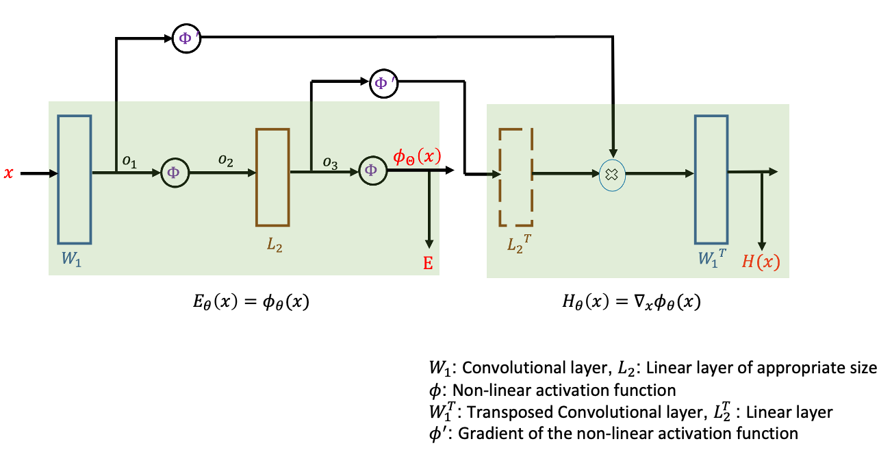
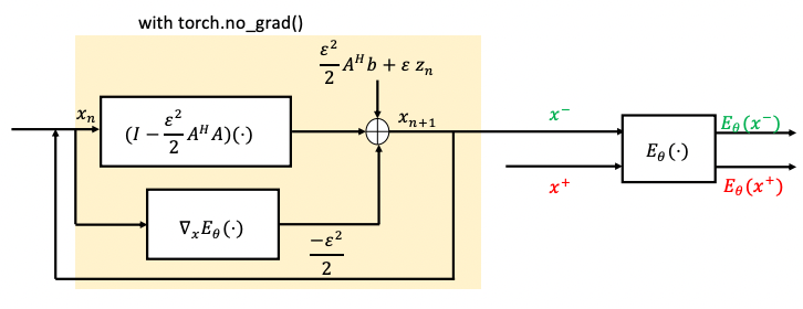
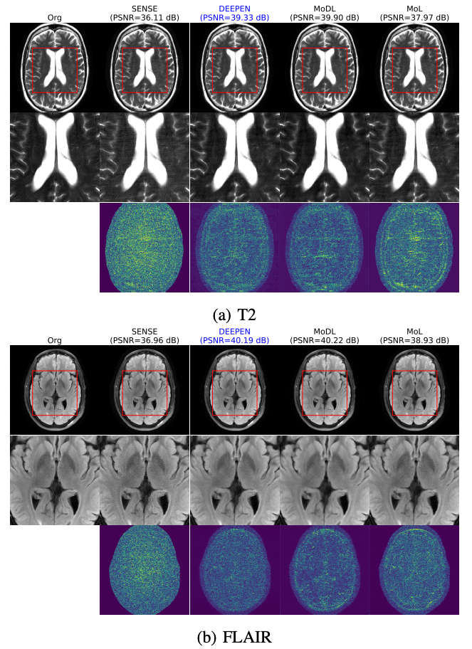
Figure 3: Comparison of the E2E MAP estimates (DEEPEN, MoDL, and its memory-efficient counterpart MoL) for two different contrasts. The top, second, and third row shows the reconstructed, enlarged, and the error image, respectively. We observe that the E2E-DEEPEN MAP estimates are comparable to MoDL, while MoL DEQ offers lower performance because of the Lipschitz constraint on the CNN.