0015
Graph Image Prior for Unsupervised Dynamic MRI Reconstruction1Tsinghua University, Beijing, China, 2School of Medicine, Chongqing University, Chongqing, China
Synopsis
Keywords: AI/ML Image Reconstruction, Machine Learning/Artificial Intelligence, Unsupervised Learning, Image Reconstruction, Dynamic MRI
Motivation: Current unsupervised dynamic-MRI reconstruction algorithms based on DIP uses very low-dimensional latent variables and a single generator for direct non-linear mapping, which may limit the performance.
Goal(s): To propose a new model and algorithm for unsupervised dynamic MRI reconstruction.
Approach: We propose a novel Graph-Image-Prior(GIP) model, which uses branched CNN generators to recover the image structure, and use a Graph-Neural-Network(GNN) to discover the best spatio-temporal manifold. Besides, we devise an ADMM algorithm to alternately optimize the dynamic image and network.
Results: The proposed method achieves the state-of-art performance even compared with supervised deep-learning methods, without the need for any fully-sampled data.
Impact: The proposed Graph-Image-Prior(GIP) scheme is a new unsupervised image reconstruction model, which has a significant value for further research. Besides, GIP is promising to be used in other multi-frame MRI reconstruction applications where fully-sampled data is scarce or unavailable.
Introduction
The inductive bias of deep convolutional-neural-network(CNN) can act as a strong regularizer for image restoration, which is known as Deep-Image-Prior(DIP)[1]. In recent years, generative models based on DIP have been demonstrated effective for unsupervised dynamic MRI reconstruction[2][3][4]. In order to exploit the spatio-temporal correlations, current algorithms usually use very low-dimensional latent variable and a single CNN generator to formulate the generative model. This may limit the algorithm performance, and increase the difficulty for network training.In this work, we propose a novel "Graph Image Prior"(GIP) scheme for unsupervised dynamic MRI reconstruction. Specifically, we decompose the generative model into two stages: "Image Recovery" and "Manifold Discovery". A noise input is fed into branched generators to recover the image structure, and then the spatio-temporal manifold is learned by a Graph-Neural-Network(GNN)[5][6]. Additionally, we devise an ADMM[7] algorithm to optimize the images and network alternately to get better results. The experiment results show that the proposed method can even outperforms the state-of-art supervised deep-learning algorithms.
Methods
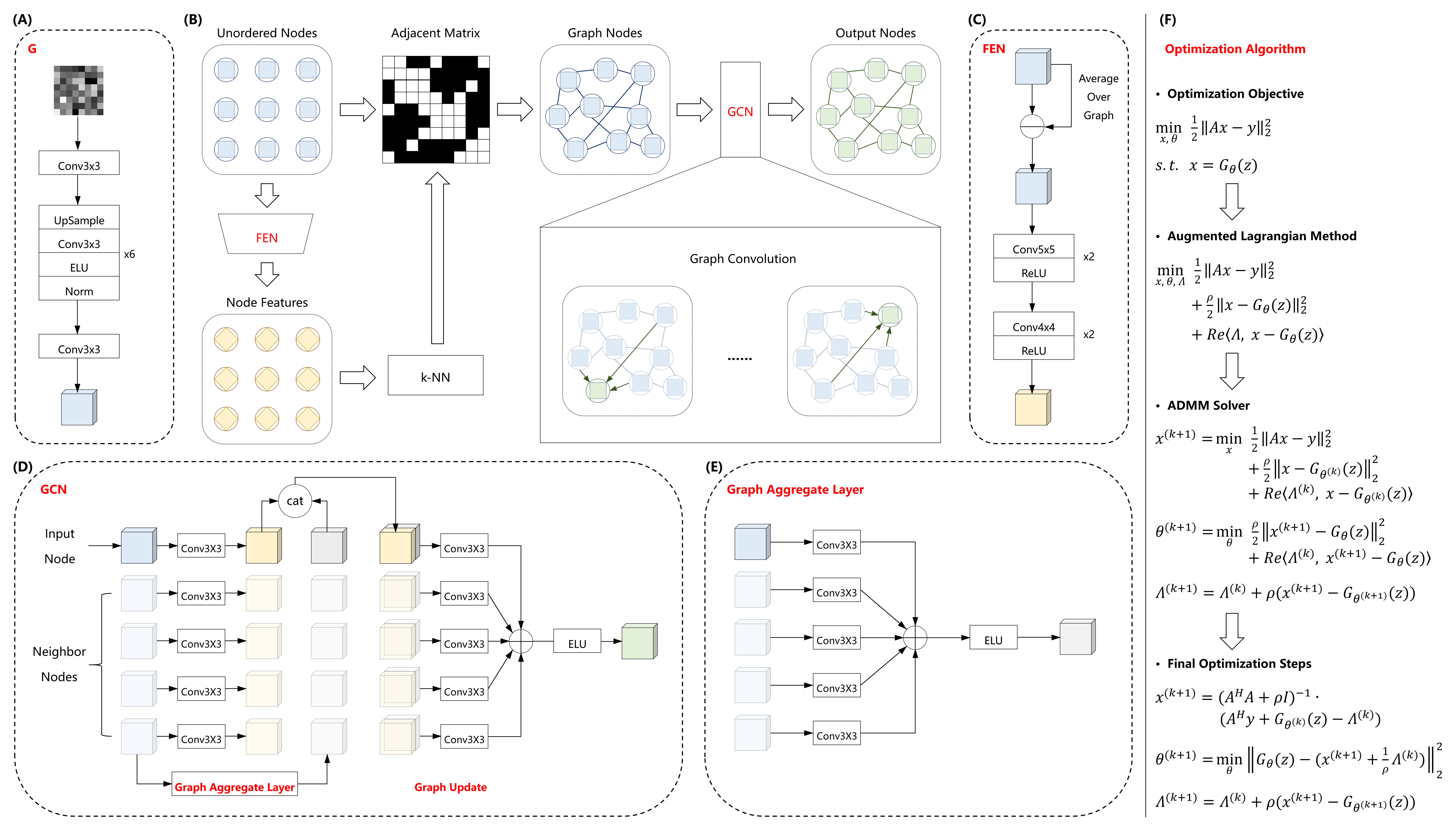
The conceptual model of GIP is illustrated in Fig1. Different from the single-generator scheme(shown in Fig1A), GIP uses independent small CNNs($$$G_{1},......,G_{N}$$$) for each frame to recover the image structure. Besides, a single 2D noise is used as input, instead of using multiple very low-dimensional latent variables. The output of the small CNNs are considered as nodes which constitute a undirected graph. A GNN[6] is used to learn the graph connections and weights to discover the most representative spatio-temporal manifold.The network structure and data-flow are illustrated in Fig2. The independent small CNN generators($$$G_{1},......,G_{N}$$$) are shown in Fig2A. The GNN layer is illustrated in Fig2B. The inputs are considered as unordered nodes, which are first fed into a Feature-Extract-Network(FEN) to obtain node features, as shown in Fig2C. K-Nearest-Neighbor(k-NN) algorithm is used to reserve the top-k neighbors for each node and build the graph adjacent matrix. The graph nodes are fed into a Graph-Convolution-Network(GCN) to update the graph. The GCN is composed of Graph-Aggregate and Graph-Update operations to learn the neighbor connections, as shown in Fig2D and Fig2E. The independent CNNs($$$G_{1},......,G_{N}$$$) and the GNN constitute the overall generator $$$G_{\theta}$$$, which is learned in a totally unsupervised manner.
Additionally, we propose to use the ADMM algorithm to improve the reconstruction performance and training convergence. Specifically, we formulate the reconstruction problem as:$$\min_{x,\theta} \frac{1}{2}\left \| Ax-y \right \|_2^2 \\s.t.\,\,x=G_{\theta}(z)$$, where $$$x$$$ is the dynamic image, $$$A$$$ is the dynamic multi-coil MRI encoding matrix, $$$z$$$ is the input noise, $$$G_{\theta}$$$ is the generator. We use augmented Lagrangian method to relax the constraints, and use ADMM solver for optimization:$$x^{(k+1)}=(A^HA+\rho I)^{-1}(A^Hy+G_{\theta^{(k)}}-\Lambda^{(k)})\\\theta^{(k+1)}=\min_{\theta} \left \| G_{\theta}(z) - (x^{(k+1)}+\frac{1}{\rho}\Lambda^{(k)}) \right \| _2^2\\\Lambda^{(k+1)}=\Lambda^{(k)}+\rho (x^{(k+1)}-G_{\theta^{(k+1)}}(z))$$, where $$$\rho$$$ is the weighting coefficient, $$$\Lambda$$$ is the Lagrangian multiplier. The optimization algorithm is explained in detail in Fig2F. Note that the second step is exactly a L2-minimization problem respect to the $$$G_{\theta}$$$ output, which can be solved by network-training. Therefore, the overall algorithm actually alternatedly optimize the dynamic image $$$x$$$ and network $$$G_{\theta}$$$.
Experiments and Results
A subset of the OCMR[8] dataset is used for reconstruction experiments, which consists of 49 fully-sampled short-axis cardiac CINE k-space data in total. The coil number are compressed to 8 by GCC[9] algorithm. The data size are all cropped to 144x144. 2D Poisson mask is used for sampling in k-space. Two acceleration factor R=8.0(ACS=10x10), R=16.0(ACS=6x6) are tested.A total of 2 traditional iterative algorithms (SToRM[10], L+S[11]), 4 supervised deep-learning agorithms (MoDL[12], SLR-Net[13], CRNN[14], L+S-Net[15]), and 1 unsupervised algorithms (TDIP[2]) are implemented for comparison. For SToRM, the ACS data is used for calculating the Laplacian matrix. For the supervised methods, each data is reconstructed by leave-one-out training strategy. All algorithms are tuned to ensure good performance. For the proposed method, we first pretrain the $$$G_{\theta}$$$ in the DIP fasion and then use ADMM algorithm with $$$\rho=0.02$$$ and 20 iterations, each with 500 network updates.
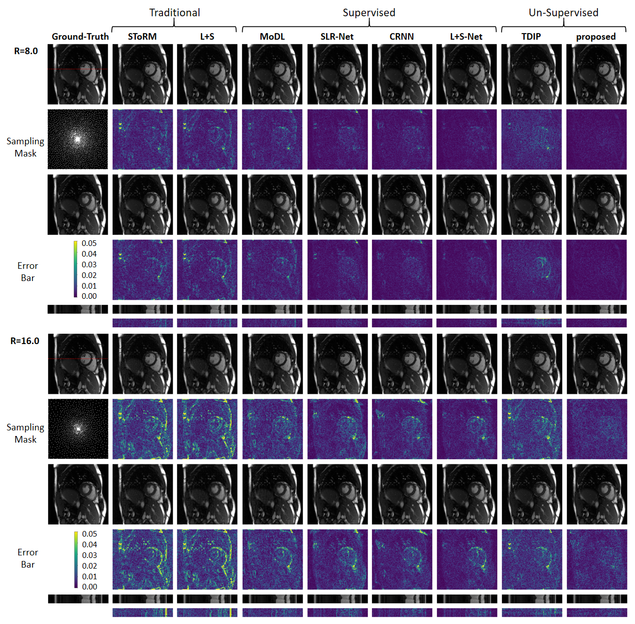
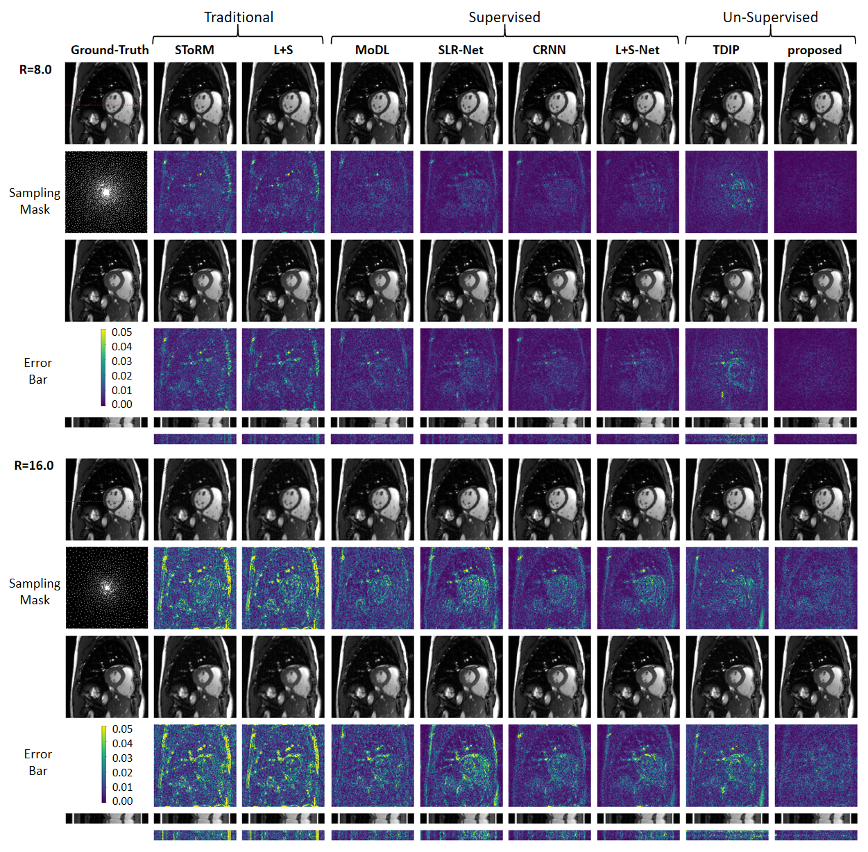
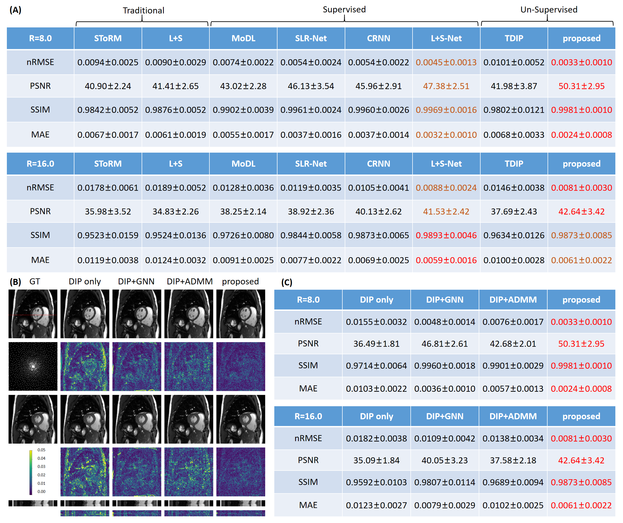
The reconstruction images are displayed in Fig3 and Fig4. The proposed method achieves the lowest reconstruction error even compared with supervised methods. The quantitative results on the whole datatset are summarized in Fig5A. Besides, ablation studies are conducted respect to the proposed method, as shown in Fig5B and Fig5C. It is shown that DIP, GNN and ADMM optimization all contribute to the improvement of reconstruction performance.
Conclusion
In this work, we propose a novel Graph-Image-Prior(GIP) scheme for unsupervised dynamic MRI reconstruction, which achieves the state-of-art performance without the need for any fully-sampled data. GIP is a promising model for other unsupervised multi-frame MRI reconstruction applications.Acknowledgements
No acknowledgement found.References
[1]. Ulyanov, D., Vedaldi, A., & Lempitsky, V. (2018). Deep image prior. In Proceedings of the IEEE conference on computer vision and pattern recognition (pp. 9446-9454).
[2]. Yoo, J., Jin, K. H., Gupta, H., Yerly, J., Stuber, M., & Unser, M. (2021). Time-dependent deep image prior for dynamic MRI. IEEE Transactions on Medical Imaging, 40(12), 3337-3348.
[3]. Zou, Q., Ahmed, A. H., Nagpal, P., Kruger, S., & Jacob, M. (2021). Dynamic imaging using a deep generative SToRM (Gen-SToRM) model. IEEE transactions on medical imaging, 40(11), 3102-3112.
[4]. Ahmed, A. H., Zou, Q., Nagpal, P., & Jacob, M. (2022). Dynamic imaging using deep bi-linear unsupervised representation (deblur). IEEE transactions on medical imaging, 41(10), 2693-2703.
[5]. Kipf, T. N., & Welling, M. (2016). Semi-supervised classification with graph convolutional networks. arXiv preprint arXiv:1609.02907.
[6]. Han, K., Wang, Y., Guo, J., Tang, Y., & Wu, E. (2022). Vision gnn: An image is worth graph of nodes. Advances in Neural Information Processing Systems, 35, 8291-8303.
[7]. Boyd, S., Parikh, N., Chu, E., Peleato, B., & Eckstein, J. (2011). Distributed optimization and statistical learning via the alternating direction method of multipliers. Foundations and Trends® in Machine learning, 3(1), 1-122.
[8]. Chen, C., Liu, Y., Schniter, P., Tong, M., Zareba, K., Simonetti, O., ... & Ahmad, R. (2020). OCMR (v1. 0)--open-access multi-coil k-space dataset for cardiovascular magnetic resonance imaging. arXiv preprint arXiv:2008.03410.
[9]. Zhang, T., Pauly, J. M., Vasanawala, S. S., & Lustig, M. (2013). Coil compression for accelerated imaging with Cartesian sampling. Magnetic resonance in medicine, 69(2), 571-582.
[10]. Poddar, S., & Jacob, M. (2015). Dynamic MRI using smoothness regularization on manifolds (SToRM). IEEE transactions on medical imaging, 35(4), 1106-1115.
[11]. Otazo, R., Candes, E., & Sodickson, D. K. (2015). Low‐rank plus sparse matrix decomposition for accelerated dynamic MRI with separation of background and dynamic components. Magnetic resonance in medicine, 73(3), 1125-1136.
[12]. Aggarwal, H. K., Mani, M. P., & Jacob, M. (2018). MoDL: Model-based deep learning architecture for inverse problems. IEEE transactions on medical imaging, 38(2), 394-405.
[13]. Ke, Z., Huang, W., Cui, Z. X., Cheng, J., Jia, S., Wang, H., ... & Liang, D. (2021). Learned low-rank priors in dynamic MR imaging. IEEE Transactions on Medical Imaging, 40(12), 3698-3710.
[14]. Qin, C., Schlemper, J., Caballero, J., Price, A. N., Hajnal, J. V., & Rueckert, D. (2018). Convolutional recurrent neural networks for dynamic MR image reconstruction. IEEE transactions on medical imaging, 38(1), 280-290.
[15]. Huang, W., Ke, Z., Cui, Z. X., Cheng, J., Qiu, Z., Jia, S., ... & Liang, D. (2021). Deep low-rank plus sparse network for dynamic MR imaging. Medical Image Analysis, 73, 102190.
Figures
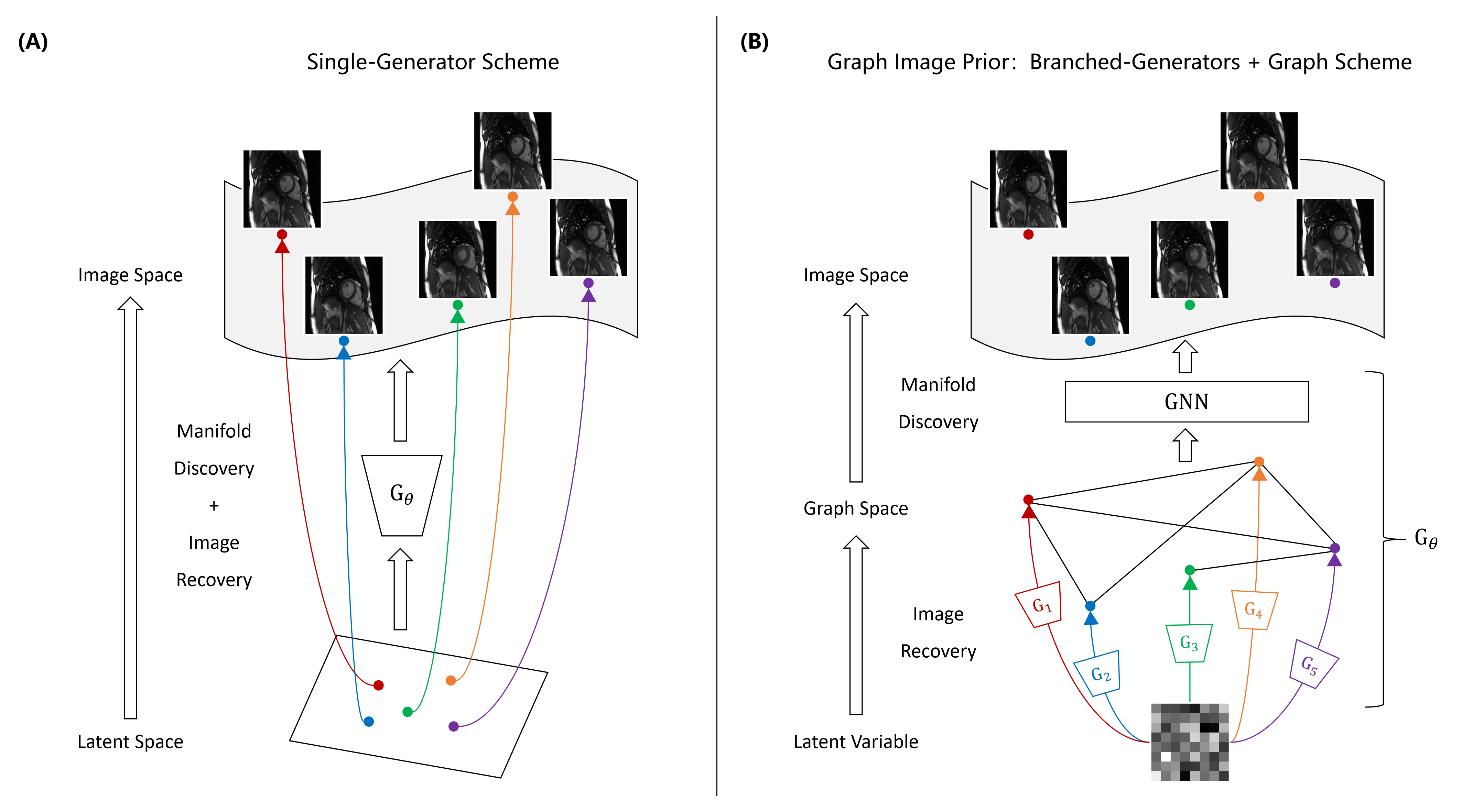
Figure 1. The conceptual model for Graph Image Prior. The single-generator scheme is shown in (A). The proposed GIP is shown in (B). GIP formulates the generative model into two stages. First, independent small CNN generators (G1,......,GN) are used for image recovery with a single 2D noise input. Second, the frames are considered as nodes, and a GNN is used for exploiting the most representative spatio-temporal manifold structure for the dynamic image. The disentanglement of image recovery and manifold discovery is beneficial for addressing the two problem better respectively.