Basic Artifacts
1Radiology, University of Cambridge, Cambridge, United Kingdom
Synopsis
Keywords: Image acquisition: Artefacts
Image artifacts can arise from one or more of the following: MR physics, MR system hardware, and the patient. Given the wide range of possible MR artifacts this presentation will be limited to the main relationships between data corruptions during image acquisition, i.e., in raw data or k-space, and their appearance in the reconstructed image after Fourier transformation. The cause and effect of artifacts including Gibbs ringing, phase encode direction aliasing/foldover, zippers, spikes and motion during image acquisition will be discussed, together with failures in fat suppression and the effect of receiver bandwidth on chemical shift artifact.Introduction
MRI is undoubtedly the most powerful and versatile diagnostic imaging method ever created. With this power, however, comes complexity and, some features in an image may be unintended, unexpected, and poorly understood. We generally refer to these features as artifacts since they may lead to interpretive difficulties or errors. The best remedy for MRI artifacts and their potential to produce diagnostic errors is to promote understanding, so that they can be prevented or, alternatively, one can potentially utilize the information content of an artifact to contribute to diagnostic content. Image artifacts can arise from one or more of the following: MR physics; MR system hardware; the patient. Given the wide range of MR artifacts I have chosen to limit this description of basic artifacts to the main relationships between data corruptions during image acquisition, i.e., in the raw data or k-space, and their appearance in the reconstructed image, i.e., after Fourier transformation. For descriptions of other artifacts, the reader is directed to the other presentations in this session as well as review articles in the literature (1-8).k-space vs. image space
To understand the cause of artifacts in reconstructed images it is necessary to understand the relationship between k-space and image space. The most common method of acquiring MR images is to use the spin-warp method (9), developed at the University of Aberdeen in 1980. Following slice selective excitation that tips the net magnetisation into the transverse plane, the spin warp method uses a variable area phase encoding gradient to impart a phase twist, or warp, to the spins in the phase encoding direction. This spatial variation in the spin phase is retained when the MR echo is digitised in the presence of the frequency encoding gradient. Each echo is then saved in the MR raw data or k-space. The echoes acquired with the smallest area, i.e., the lowest ± amplitude phase encoding gradients, that impart a 2π phase twist across the phase field-of-view ($$$FOV_y$$$), are placed either side of the centre of k-space, i.e., at the $$$± 1\: k_y$$$ lines. The echoes acquired with the largest ± amplitude phase encoding gradients, that impart a 2π phase shift across adjacent voxels, are placed at either end of k-space, i.e., $$$± k_{y,max}/{2}$$$. The other phase encoding gradient areas are linearly scaled between these two extremes, such that the difference between adjacent phase encoding steps $$$\Delta k\ =1/{FOV_y}$$$, and $$$k_{y,max}=\frac{1}{2}(N_y-1)\Delta k_y$$$, where $$$N_y$$$ is the number of phase encoding steps. The maximum area of the phase encoding gradient is given by $$$A_{y,max}=\frac{\ 2\pi\ (N_y-1)}{\ \gamma\ FOV_y}$$$. Following phase encoding the echo signal is then frequency encoded in the orthogonal direction. The frequency encoding gradient causes the phase encoded spins to precess at spatially varying frequencies along the direction of the gradient. Defining the spatial frequencies $$$ k_x=\gamma\int{G_x\left(t\right)}\: dt$$$ and $$$ k_y=\gamma\int{G_y\left(t\right)}\: dt$$$, then for simple constant amplitude gradients the signal can be written as $$$S\left(k_x,k_y\right)=\iint{\rho\left(x,y\right)e^{-ik_xx}e^{-ik_yy}dxdy}$$$, where $$$\rho\left(x,y\right)$$$ is the effective spatial distribution of the proton density of the tissues. Hence the use of the spin -warp method means that image reconstruction can be directly performed using a 2D inverse Fourier transform. The inverse relationship between k-space and image space (Figure 1) means that the spacing between phase encode steps ($$$\Delta k_y$$$) or frequency encode samples ($$$\Delta k_x$$$) dictates the field-of-view (FOV) in the phase encode and frequency encoding direction respectively. Similarly, this inverse relationship means that the spatial resolution in the phase encode direction is dictated by the extent of k-space, i.e.,$$$\Delta y=1/2k_{y,max}$$$ , with a similar equation for the spatial resolution in the frequency encoding direction.Gibbs ringing
The Fourier transform assumes that the signal being transformed is periodic and extends infinitely in all directions. However, in practice, the acquired MRI data has a finite extent and is truncated in comparison to the idealised situation. The consequence of this truncation is that the Fourier transform cannot accurately represent the transition of a signal with a sharp discontinuity, such as an edge. The Gibbs phenomenon is a well-known mathematical property where, during the Fourier transformation of a signal with such a sharp discontinuity, oscillatory overshoots or undershoots occur near the transition region. These oscillations manifest as bright and dark lines parallel to, but decaying in amplitude with distance from, the discontinuity. In the spatial domain, this is known as Gibbs ringing (Figure 2). Josiah Willard Gibbs was Professor of mathematical physics at Yale from 1871 until his death in 1903. Working in relative isolation, he became the earliest theoretical scientist in the United States to earn an international reputation and was praised by Albert Einstein as "the greatest mind in American history”. In 1899, inspired by correspondence in Nature between A. A. Michelson (Chicago) and A. E. H. Love (Oxford) about the convergence of the Fourier series of the square wave function, Gibbs (after making a mistake in his initial communication) eventually described this overshoot at the point of a discontinuity (10). In 1906, the American mathematician Maxime Bôcher gave a detailed mathematical analysis of the overshoot, coining the term "Gibbs phenomenon" (11) and bringing the term into widespread use. To mitigate Gibbs ringing, one common approach is to apply a low-pass filter to the raw k-space data that reduces the amplitude of the high-frequency components at the edge of k-space. This data apodisation can help reduce the ringing, but at the cost of some loss of sharpness or fine details in the reconstructed image. Alternatively higher spatial frequencies can be acquired, i.e., more $$$N_x$$$ and/or $$$N_y$$$ samples can be acquired, resulting in a smaller voxel size and hence a higher spatial resolution. This has the effect of moving the oscillations towards the discontinuity but does not decrease their magnitude.Phase-encode direction aliasing or foldover
MRI allows different FOVs to be selected in the frequency and phase encoding direction. In the frequency encoding direction, the FOV and the readout (receiver) bandwidth are selected by the operator. These two pieces of information allow the system to calculate the desired frequency encoding gradient strength. The readout bandwidth information is also used by the system to electronically filter out any frequencies outside of the bandwidth. However, in the phase encoding direction, the signal encoding is achieved through the phase imparted to the spins (9), so there is no direct analogue to frequency filtering. The desired phase FOV can also be chosen by the operator but in this case any tissue that exists outside this FOV will be encoded incorrectly. The minimum ± phase encoding gradient amplitudes are calculated to achieve a 2π phase shift across the selected FOV. This means that any tissue beyond the FOV will be phase aliased (Figure 3). For example, if the FOV is 30cm then tissue at 32cm will appear at 2cm, i.e., it will appear on the other side of the image. Usually, phase encode aliasing, sometimes known as foldover, is easy to recognize, but the resulting image can be confusing if the aliased body part is completely outside the FOV so that continuity from one side of the image to the other is difficult to recognize. Examples include an arm or hand mimicking a lesion or enhancing vessels in the mediastinum resembling an enhancing tumour in the breast. Simply swapping the phase and frequency directions, so that all the tissue along the phase axis is within the FOV may be sufficient to eliminate these artifacts. However, if there are good reasons to place the direction of the phase encoding axis along the long axis of the patient, e.g., to control the direction of motion artifacts (see Patient motion below), or if both axes extend beyond the desired FOV then it may be necessary to employ no-phase-wrap techniques. These methods extend the original FOV in the phase encode direction, commonly by a factor of two, whilst commensurately reducing the number of signal averages to maintain the pixel size and signal-to-noise ratio. Tissue signal outside of the extended FOV aliases into the regions of extended FOV and are discarded resulting in the original FOV image being displayed but without any aliasing artifact. However, if the body part is sufficiently large, aliasing may still degrade an image. With 3D Fourier transform acquisitions, a second orthogonal phase encoding gradient is used to encode slices. Even though the excitation is often slab selective the profile of the excitation slab is not sharp at the edges, which means that some signal will be excited outside the range of the slice axis phase encoding. Therefore, data can be aliased in this direction as well as the axis of in-plane phase encoding. Because the aliased structures are at a level distant from the reconstructed image, this form of phase aliasing can be more confusing to understand. Viewing the top and bottom slices can usually clarify this artifact.RF interference/zipper artifacts
Many image artifacts result from undesired RF signals that corrupt the MR data. This undesired RF may arise externally or internally to the MR system. External sources are usually minimized by locating the magnet inside an RF shielded enclosure or cabin. This cabin provides a high degree of immunity from external interference and prevents leakage of the high-power RF from the MR system. However, if there is a problem with this enclosure then external RF can enter the MR receiver system. If this interference is periodic with either single or multiple frequencies, then the artifact typically appears as a bright and dark alternating pattern in the phase encoding direction that is often referred to as a zipper artifact. A more uncommon form of zipper artifact may be seen parallel to the frequency encoding direction along a line at magnet isocentre (Figure 4). This artifact may be seen with spin echo-based sequences and is due to the transverse magnetisation created by the imperfect 180°. This free induction decay (FID) signal may then overlap the beginning of the digitised spin echo signal. Since this FID is created after phase encoding its amplitude is constant during each phase encoding, i.e., it can be considered as a DC offset. Following Fourier transformation this DC offset manifests as a line through the centre of the gradient field, i.e., not necessarily through the centre of the image. The FID is usually “crushed” by applying balanced dephasing gradient lobes either side of the 180° slice selection gradient, with the gradient lobe on the right doing the dephasing and the gradient on the left balancing the phase shift imparted by the right lobe. In addition, the RF excitation pulse is usually “chopped”, i.e., the 90° excitation pulse has a 180° phase shift applied on alternate TRs. This has the effect of pushing the DC artifact to the edges of the image FOV, where the images lines can be blanked if required.Spike noise
The periodic RF interference described above should be contrasted with short intense artifacts that affect only single points in k-space, called “spike-noise” or “white pixel noise” (12). One or more spikes of detected external noise may produce a patterned degradation of the image. Depending upon where this point occurs in k-space the overall image, after Fourier transformation, will demonstrate a superimposed banding artifact corresponding to that spatial frequency (Figure 5). A spike occurring near the centre of k-space will have a low frequency banding whilst a spike occurring near the edge of k-space will generate a high frequency banding. This cross-hatching appearance is sometimes referred to as a corduroy (single spike) or herringbone (multiple spikes) artifact. Causes of such artifact can include static electricity from clothing or blankets, or random noise from electrical sources such as damaged filament light bulbs, or electrical discharges from gradient cable connections.Patient motion
The MRI acquisition process assumes that the underlying tissue does not change in location or signal intensity during the acquisition. Any changes can cause modulation of the MRI signal, creating artifacts (13, 14). Since a single frequency encoding is very rapid, motion does not generally cause artifacts in the frequency encoding direction. However, the interval between phase encoding steps in a conventional sequence, i.e., every TR, is more temporally commensurate with the rates of physiological motion. Hence motion artifacts, regardless of the direction of the motion, will manifest as artifacts in the phase encoding direction, usually as “ghosting” whereby replicates of the moving structure are propagated along the phase encoding direction. Any type of movement can give rise to such ghosting appearances, including whole body motion, respiration, cardiac motion, and blood flow. Many artifact reduction strategies focus on either removing the motion (e.g., breath-holding), compensating for the motion (e.g., ECG-triggering, respiratory triggering, or reordering phase encoding), suppressing the signal of moving tissue, e.g., spatial saturation (15), signal averaging (16) or by using rapid imaging techniques. In some situations, it may be possible to swap the phase and frequency directions (see Phase-encode direction aliasing above) to change the direction of the artifact and stop it from overlying a particular area of interest. Respiratory motion causes an anterior-posterior motion of the chest wall (in-plane) as well as inferior-superior motion of the liver (through-plane) resulting in a modulation of the MRI signal amplitude with time. After Fourier transformation this modulated signal results in “sidebands” or ghosts, with the spacing of the ghosts proportional to the periodicity of the motion and inversely proportion to the TR. These sidebands appear as ghosts in the reconstructed image (Figure 6). Note that with the use of surface coil arrays the signal from subcutaneous fat is very high and can exacerbate the appearance of the ghosts. Similar amplitude modulation artifacts result from pulsatile flow in a vessel (17). Although the vessel itself is not moving the changing signal intensity with differential flow related signal enhancement throughout the cardiac cycle result in ghosting artifacts. It should also be noted that any system hardware instabilities can also cause signal modulation and hence ghosting in images. Another category of motion induced artifact that can cause signal loss and ghosting arises from the phase shifts accumulated by spins moving during the application of the imaging gradients (18). This category of motion artifact can be greatly reduced by using gradient moment nulling techniques, called flow-compensation by some vendors, which involves using more complex gradient waveforms, usually on the slice select and frequency encoding axes, so that the phase accumulated by moving spins is zero, or nulled, at the end of the gradient waveform (19, 20). The simplest form of gradient moment nulling involves correcting the phase shift due to spins moving with a constant velocity, known as the first order moment, which is the largest source of phase errors (Figure 7). Compensating for higher orders of motion, such as acceleration or jerk, requires more complex and longer duration gradient waveforms, meaning that they may cause more problems than they address. It should be noted that even complete correction of gradient moment errors does not affect amplitude modulation, so that ghosting is still likely from pulsatile flow. Some forms of motion artifact result from changes in tissue position that do not necessarily interfere with the process of phase encoding, and therefore do not produce ghost artifact along the phase encoding axis. As with any method of imaging, including conventional radiography, motion during image acquisition can produce artifacts. For example, image blurring or complex signal may occur when tissue occupies various positions during the period of image acquisition.Chemical shift selective fat saturation failure
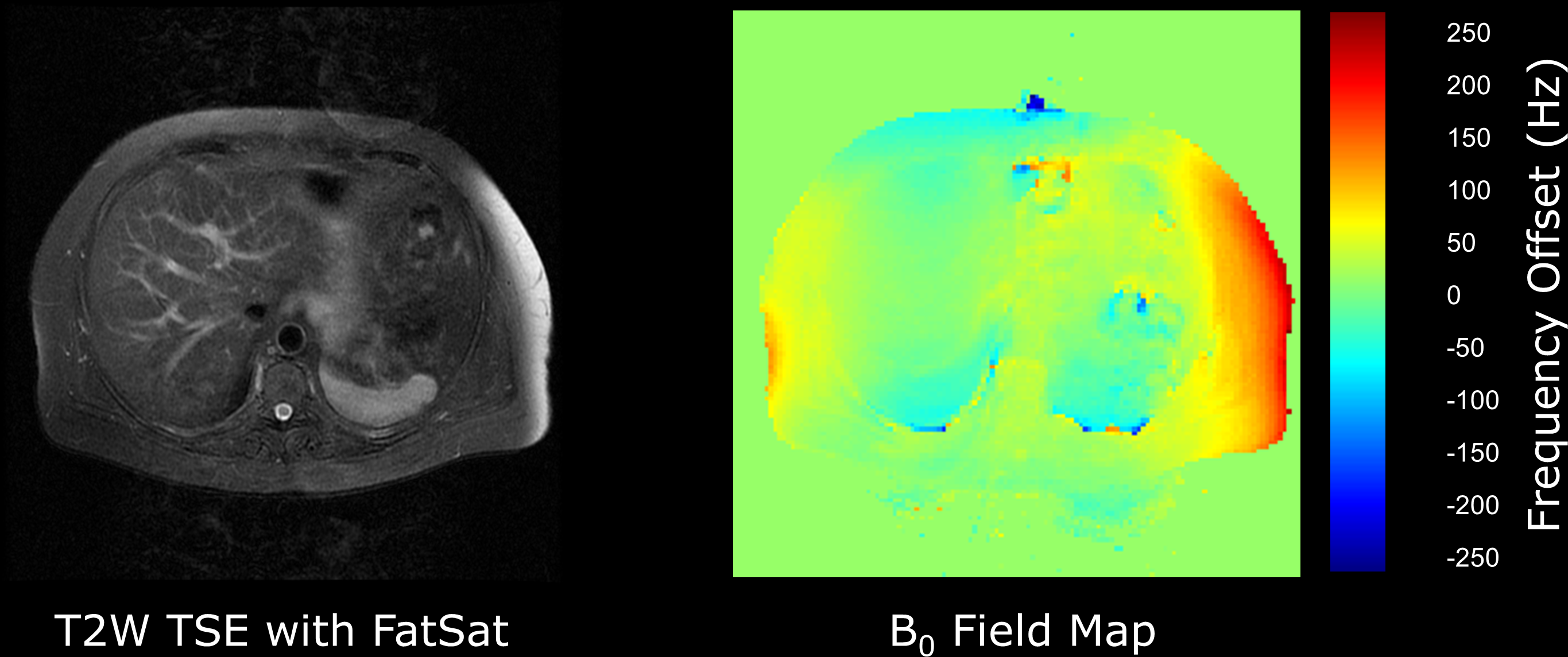
A good static magnetic field (B0) uniformity is required for all MR imaging. Manufacturing tolerances and the local installation environment means that the main magnetic field needs to be optimized at installation by the manufacturer who “shims” the magnet either passively, using small pieces of metal distributed around the room temperature bore of the magnet, or actively by adjusting the currents through additional superconducting coils within the magnet cryostat. Magnetic field uniformity is usually reported as the root mean square (rms) variation from the nominal field strength, e.g., 3.0 T, in either parts-per-million (ppm), or as a frequency variation in Hz, over many points within a given diameter spherical volume (DSV). A typical 3.0 T manufacturer’s shim would have a rms value of 50 Hz or 0.4 ppm over a 45 cm DSV. Since heterogeneous susceptibility within the human body will affect local magnetic field uniformity, manufacturers also provide methods of patient specific shimming. This involves rapidly mapping the static magnetic field uniformity, usually using a gradient echo-based phase difference technique, and adjusting the offsets on the x, y and z gradients to remove any linear field variations (21). Some systems may be equipped with additional room-temperature, i.e., non-superconducting, higher order shim coils that can further improve the uniformity, particularly over small volumes. Uniformity of B0 is important for chemical shift selective fat saturation techniques. Human adipose tissue is composed primarily of triglycerides, which are a subgroup of lipid molecules. Triglycerides comprise multiple groups of protons (CH3, CH2, CH=CH, etc) with the nuclear shielding effect resulting in a range of chemical shifts from 0.9 to 5.3 ppm lower than the water (H20) proton resonance. The most abundant triglyceride resonance comes from the methylene (CH2) groups, in which the protons resonate at approximately 3.4 ppm lower than those in water. Hence at 1.5 T the methylene peak appears at 3.4 ppm * 64 MHz = 220 Hz lower than the water resonant frequency. Chemical shift selective saturation pulses at 1.5 T are therefore centred around -220 Hz from water. These pulses have a bandwidth that is sufficiently narrow to avoid saturating the water signal. A typical 1.5 T chemical shift saturation pulse has a bandwidth of approximately 150 Hz. Therefore, to obtain good fat saturation, it is necessary that the main magnetic field does not vary by more than 150 Hz across the entire field-of-view and across all slices in a multi-slice acquisition. If this is not the case the fat saturation will be suboptimal (Figure 8). Magnetic field non-uniformity due to patient susceptibility is particularly problematic at air tissue interfaces, which are especially abundant in various locations within the chest, including the breast. Failure of fat saturation is almost inevitable when the air tissue interface is oriented along the z-axis of the magnetic field (22-24). One particularly common example is adipose tissue situated anterior to the liver, immediately inferior to the lung base. Heterogeneous susceptibility within the patient can also cause the water frequency to be shifted so that it falls within the bandwidth of the fat saturation pulse. In this situation the water signal can also become saturated. This effect has also been reported in contrast-enhanced thoracic angiography (25).Chemical shift artifact
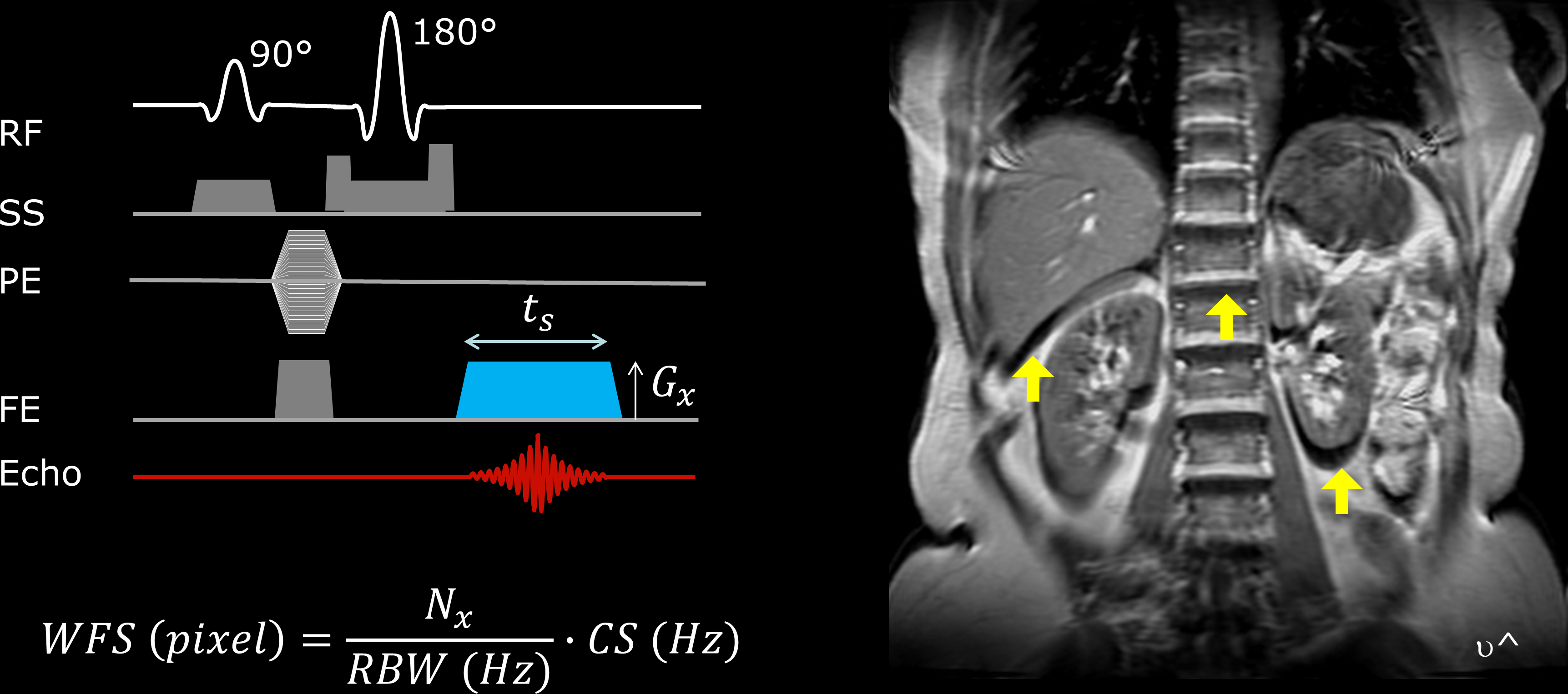
The frequency encoding gradient is used to spatially localize signals based on their precessional frequency. The natural difference in frequency of 3 ppm between the protons in water and fat means that after Fourier transformation they will be spatially shifted in the frequency encoding direction (Figure 9) (26, 27). The amount of shift will depend upon the receiver bandwidth per pixel and the chemical shift at the given field strength. For example, a typical receiver bandwidth of ±16 kHz over 256 pixels in the frequency encoding direction is equivalent to $$$32000/256 = 125 Hz/pixel$$$. At 1.5 T the chemical shift induced frequency offset is approximately 220 Hz (see Chemical shift selective fat saturation failure above), so water and fat will be spatially shifted by $$$220/125 = 1.76\: pixels$$$. Reducing the receiver bandwidth will increase the chemical shift offset and vice versa. Note that moving from 1.5 T to 3.0 T will double the offset for a given bandwidth.Summary
Image artifacts usually arise during MR acquisition; therefore, it is important to have a good understanding of the relationship between raw data, or k-space and their appearance in the reconstructed image after the inverse Fourier transformation. Artifacts can arise from one or more of MR physics, the MR system hardware, as well as the patient.Acknowledgements
Thanks to colleagues at the University of Cambridge Department of Radiology and the Cambridge University Hospitals Department of Imaging.References
- Bellon EM, Haacke EM, Coleman PE, Sacco DC, Steiger DA, Gangarosa RE. MR artifacts: a review. Ajr. 1986;147(6):1271-81.
- Bernstein MA, Huston J, 3rd, Ward HA. Imaging artifacts at 3.0T. J Magn Reson Imaging. 2006;24(4):735-46.
- Mirowitz SA. MR imaging artifacts. Challenges and solutions. Magnetic resonance imaging clinics of North America. 1999;7(4):717-32.
- Morelli JN, Runge VM, Ai F, Attenberger U, Vu L, Schmeets SH, et al. An image-based approach to understanding the physics of MR artifacts. Radiographics. 2011;31(3):849-66.
- Stadler A, Schima W, Ba-Ssalamah A, Kettenbach J, Eisenhuber E. Artifacts in body MR imaging: their appearance and how to eliminate them. European radiology. 2007;17(5):1242-55.
- Zhuo J, Gullapalli RP. AAPM/RSNA physics tutorial for residents: MR artifacts, safety, and quality control. Radiographics. 2006;26(1):275-97.
- Graves MJ, Mitchell DG. Body MRI artifacts in clinical practice: a physicist's and radiologist's perspective. J Magn Reson Imaging. 2013;38(2):269-87.
- Krupa K, Bekiesinska-Figatowska M. Artifacts in magnetic resonance imaging. Pol J Radiol. 2015;80:93-106.
- Edelstein WA, Hutchison JM, Johnson G, Redpath T. Spin warp NMR imaging and applications to human whole-body imaging. Physics in medicine and biology. 1980;25(4):751-6.
- Gibbs JW. Fourier's Series. Nature. 1899(April 27):606.
- Bôcher M. Introduction to the theory of Fourier's series. Annals of Mathematics. 1906;7(3):81-152.
- Foo TF, Grigsby NS, Mitchell JD, Slayman BE. SNORE: spike noise removal and detection. IEEE transactions on medical imaging. 1994;13(1):133-6.
- Barish MA, Jara H. Motion artifact control in body MR imaging. Magnetic resonance imaging clinics of North America. 1999;7(2):289-301.
- Wood ML, Henkelman RM. MR image artifacts from periodic motion. Medical physics. 1985;12(2):143-51.
- Felmlee JP, Ehman RL. Spatial presaturation: a method for suppressing flow artifacts and improving depiction of vascular anatomy in MR imaging. Radiology. 1987;164(2):559-64.
- Gazelle GS, Saini S, Hahn PF, Goldberg MA, Halpern EF. MR imaging of the liver at 1.5 T: value of signal averaging in suppressing motion artifacts. Ajr. 1994;163(2):335-7.
- Perman WH, Moran PR, Moran RA, Bernstein MA. Artifacts from pulsatile flow in MR imaging. Journal of computer assisted tomography. 1986;10(3):473-83.
- van Dijk P. Direct cardiac NMR imaging of heart wall and blood flow velocity. Journal of computer assisted tomography. 1984;8(3):429-36.
- Ehman RL, Felmlee JP. Flow artifact reduction in MRI: a review of the roles of gradient moment nulling and spatial presaturation. Magn Reson Med. 1990;14(2):293-307.
- Haacke EM, Lenz GW. Improving MR image quality in the presence of motion by using rephasing gradients. Ajr. 1987;148(6):1251-8.
- Schneider E, Glover G. Rapid in vivo proton shimming. Magn Reson Med. 1991;18(2):335-47.
- Anzai Y, Lufkin RB, Jabour BA, Hanafee WN. Fat-suppression failure artifacts simulating pathology on frequency-selective fat-suppression MR images of the head and neck. AJNR Am J Neuroradiol. 1992;13(3):879-84.
- Axel L, Kolman L, Charafeddine R, Hwang SN, Stolpen AH. Origin of a signal intensity loss artifact in fat-saturation MR imaging. Radiology. 2000;217(3):911-5.
- Yoshimitsu K, Varma DG, Jackson EF. Unsuppressed fat in the right anterior diaphragmatic region on fat-suppressed T2-weighted fast spin-echo MR images. J Magn Reson Imaging. 1995;5(2):145-9.
- Siegelman ES, Charafeddine R, Stolpen AH, Axel L. Suppression of intravascular signal on fat-saturated contrast-enhanced thoracic MR arteriograms. Radiology. 2000;217(1):115-8.
- Babcock EE, Brateman L, Weinreb JC, Horner SD, Nunnally RL. Edge artifacts in MR images: chemical shift effect. Journal of computer assisted tomography. 1985;9(2):252-7.
- Dwyer AJ, Knop RH, Hoult DI. Frequency shift artifacts in MR imaging. Journal of computer assisted tomography. 1985;9(1):16-8.
Figures
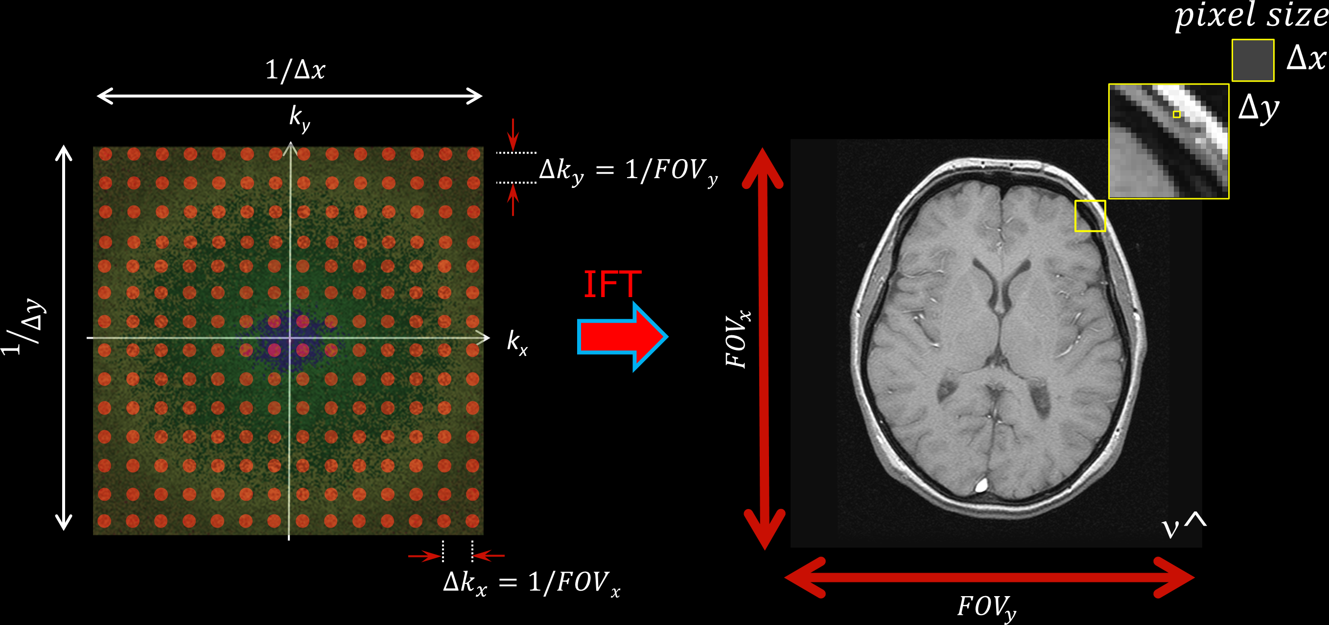
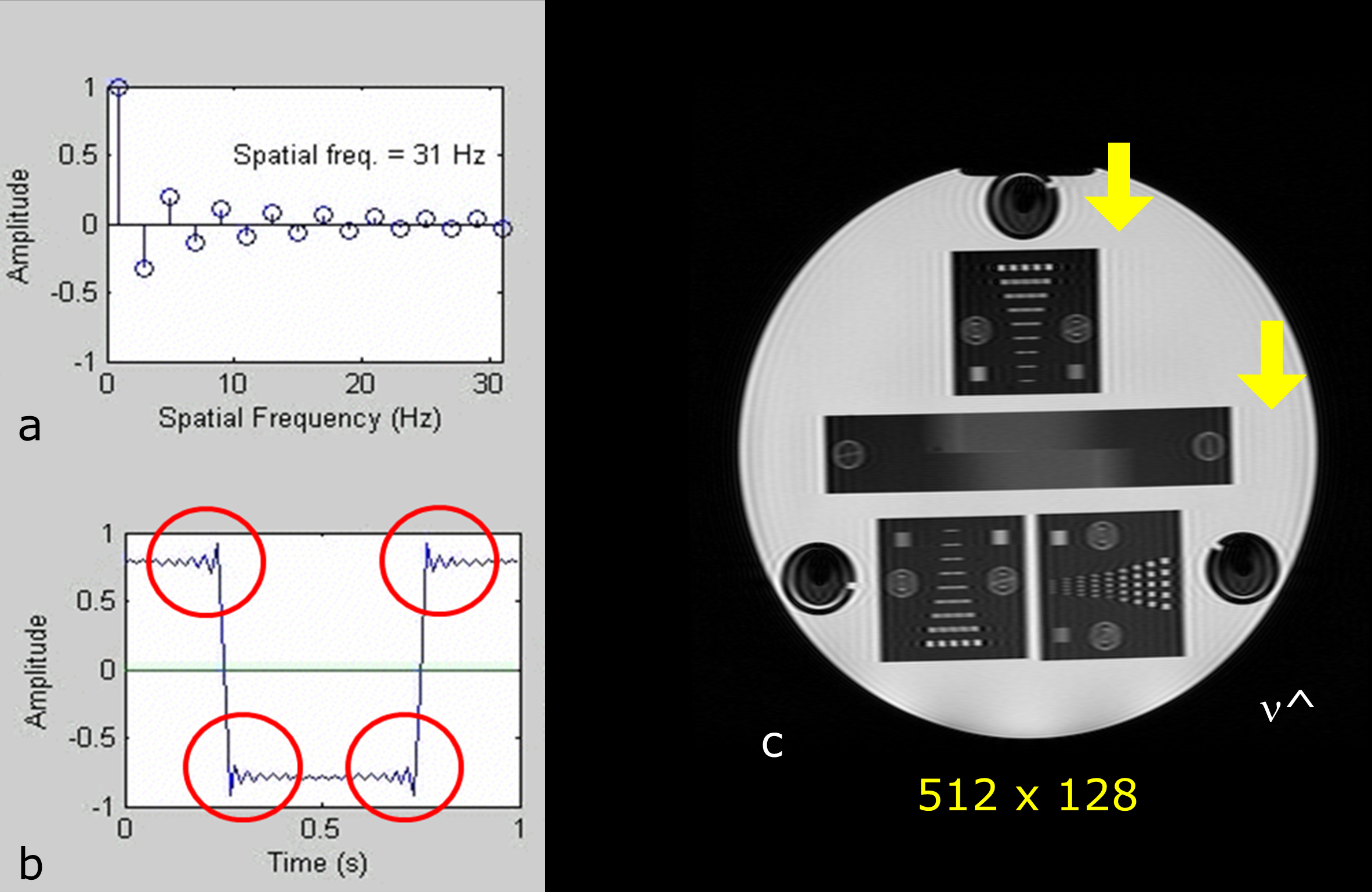
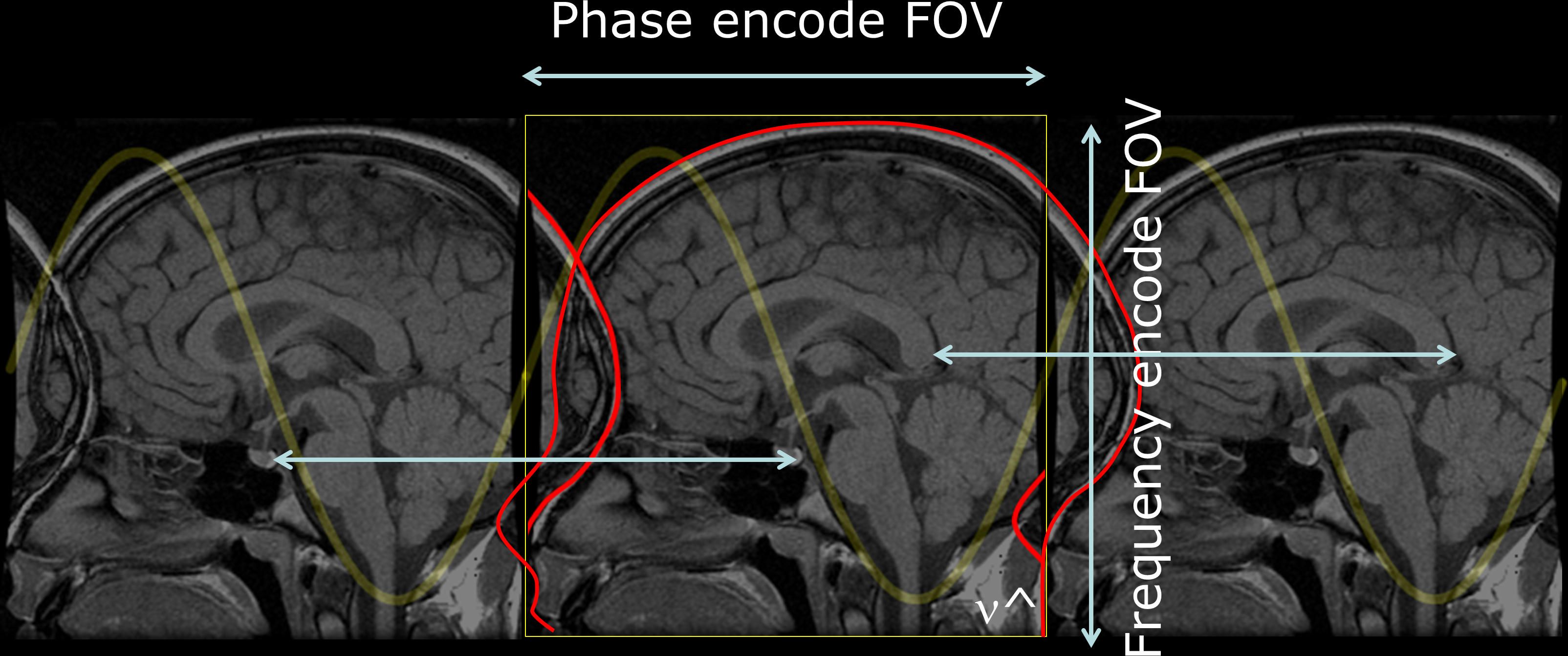
Figure 3. Phase encode direction aliasing.The 2π phase variation (sinusoid) is shown in the phase encode direction (horizontal). Replicates of the image are shown to demonstrate the phase aliasing. Any point outside the phase encode field-of-view (FOV) will have the same phase inside the imaging FOV. Features outside the FOV will be wrapped, or folded-over, into the FOV. The red outline shows the nose and back of the head wrapped back into the FOV. The spatial frequencies in the frequency encoding direction (vertical), are electronically filtered so there is no wrap in that direction.
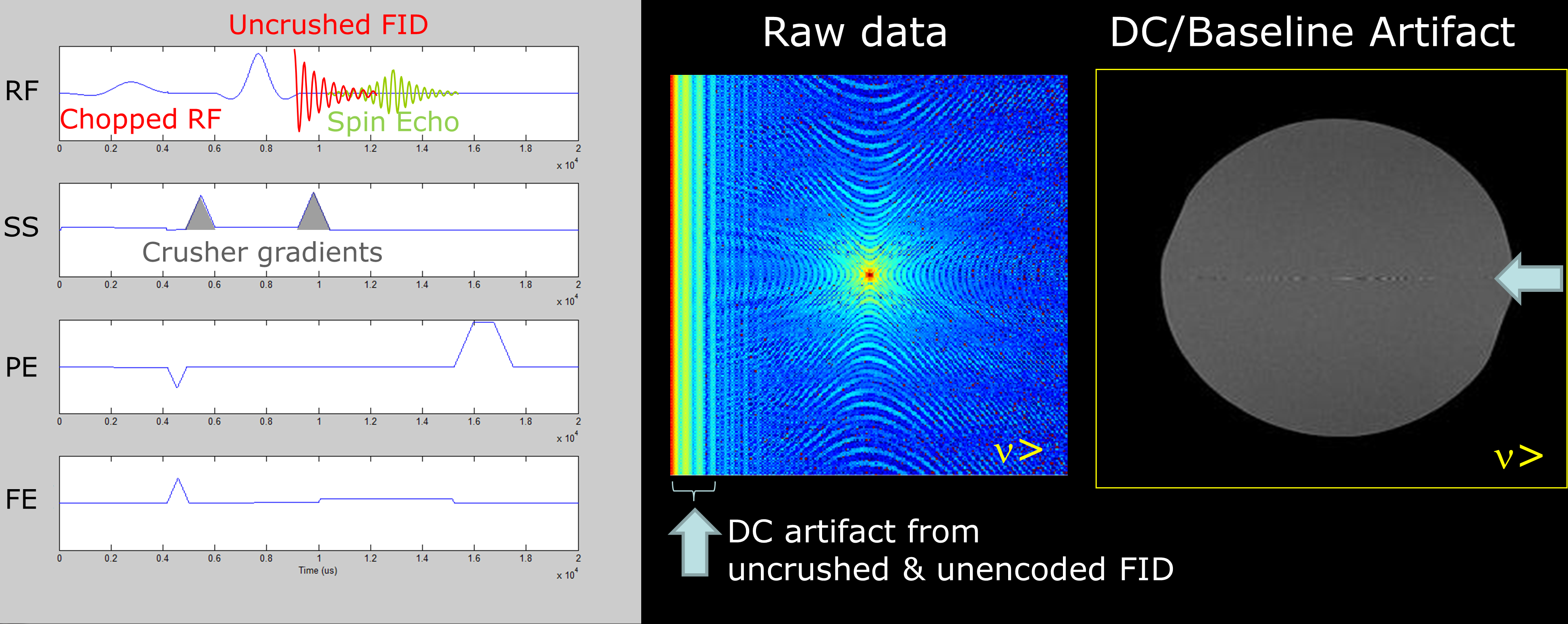
Figure 4. DC artifact. This artifact may be seen with spin echo-based sequences and arises from the free induction decay (FID), created by an imperfect 180°. The FID overlaps the spin echo and is considered a DC offset in k-space. Following Fourier transformation this DC offset manifests as a "zipper" through the centre of the gradient field (arrowed) in the frequency encoding direction. Balanced gradient lobes either side of the 180° slice select gradient are used to "crush" the FID. In addition, the RF excitation pulse is usually “chopped”, pushing the DC artifact to the edges of the FOV.
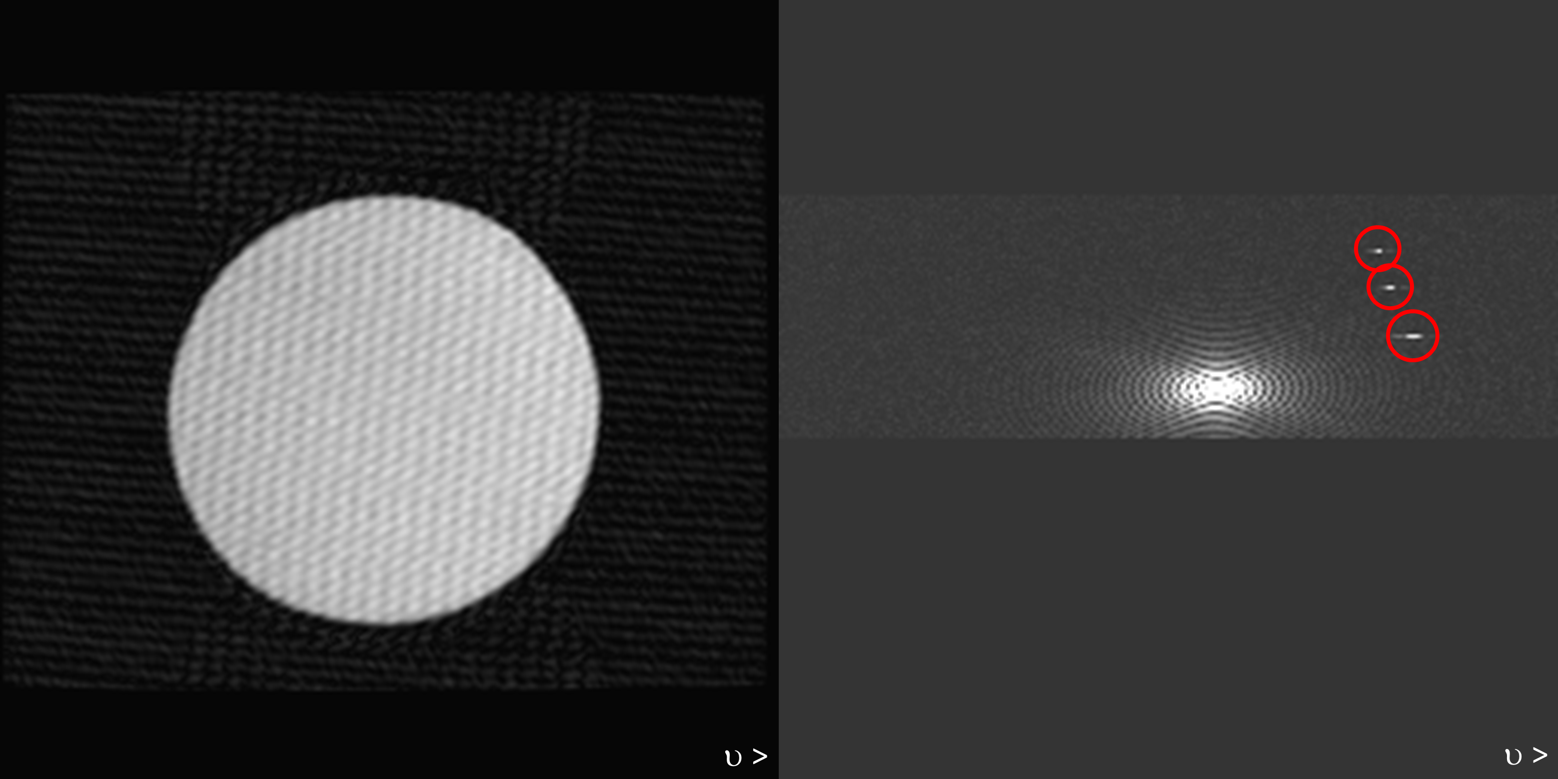
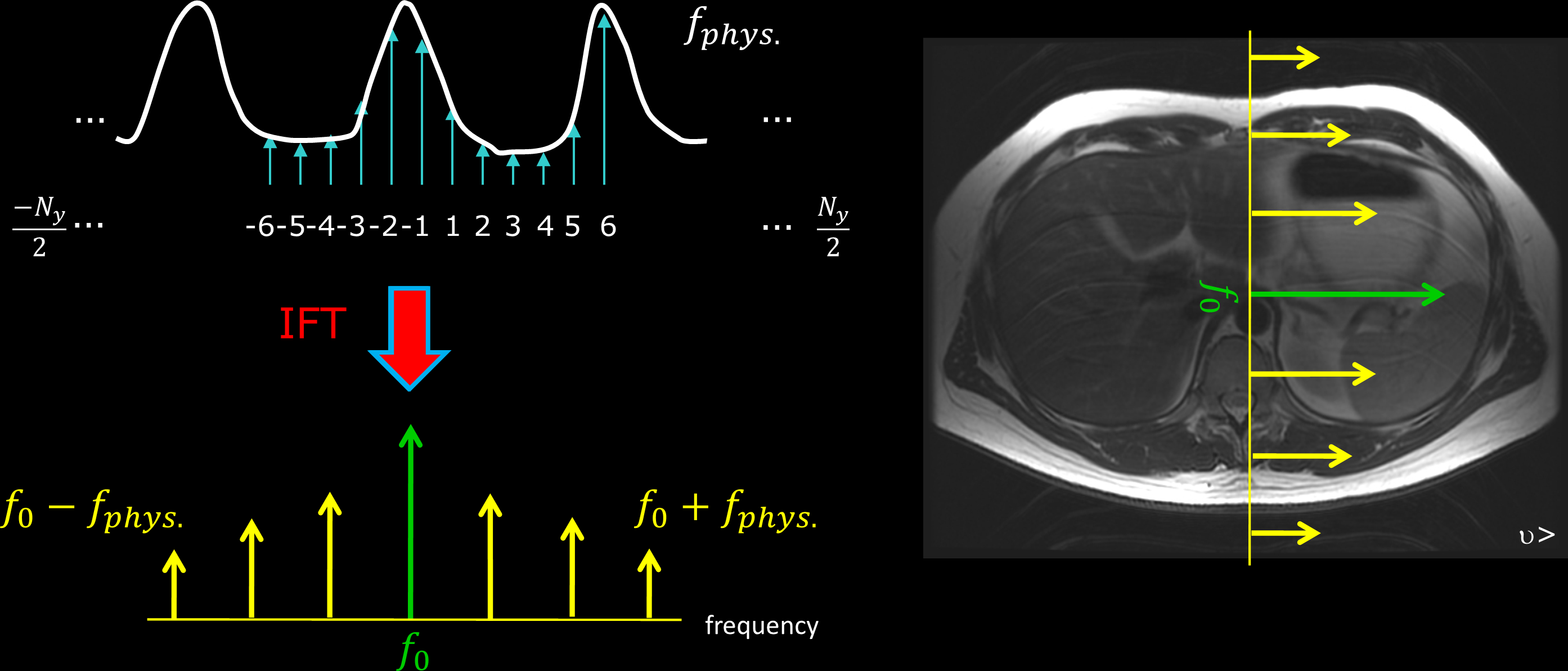
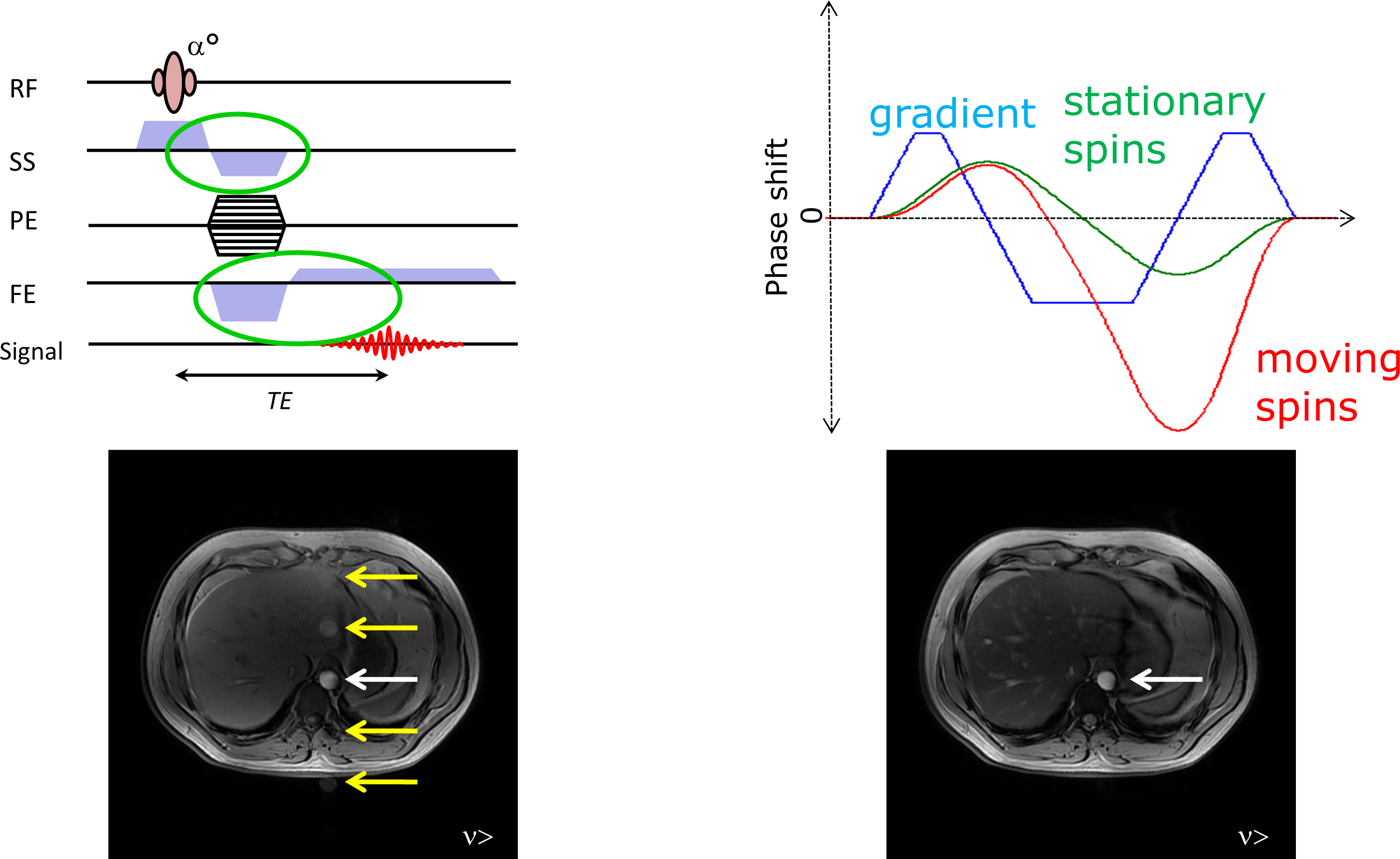
Figure 7. Flow ghosting. Top right the slice select and frequency encoding gradients have a rewinder and a pre-phaser respectively so that there is zero phase shift for stationary spins. However, flowing spins will result in a non-zero phase shift. The variable phase shifts caused by pulsatile flow result in "ghost" replicates of the vessel (bottom left image). Using a three-lobed gradient with areas 1:-2:1 (top right), results in zero phase shift for both stationary and spins moving with a constant velocity. This eliminates the flow ghosting as shown in the bottom right image.