Synopsis

Keywords: Physics & Engineering: Physics, Physics & Engineering: Pulse design, Physics & Engineering: Hardware

While the origins of MRI date from the origins of NMR in 1948, nothing much happened until Lauterbur’s 1973 paper in Nature. Even so, this was more of an idea than a reduced-to-practice methodology. It took another decade to work-out spatial localization, add the pulse FT method, and properly configure selective excitation pulses and phase-encoding gradients. Basically, a whole tool-set for manipulating NMR signals in space and time was developed to engineer the desired image response. But MRI still would not have happened, if not for the unsung revolution in magnet, and gradient and RF coil technologies.

SYLLABUS

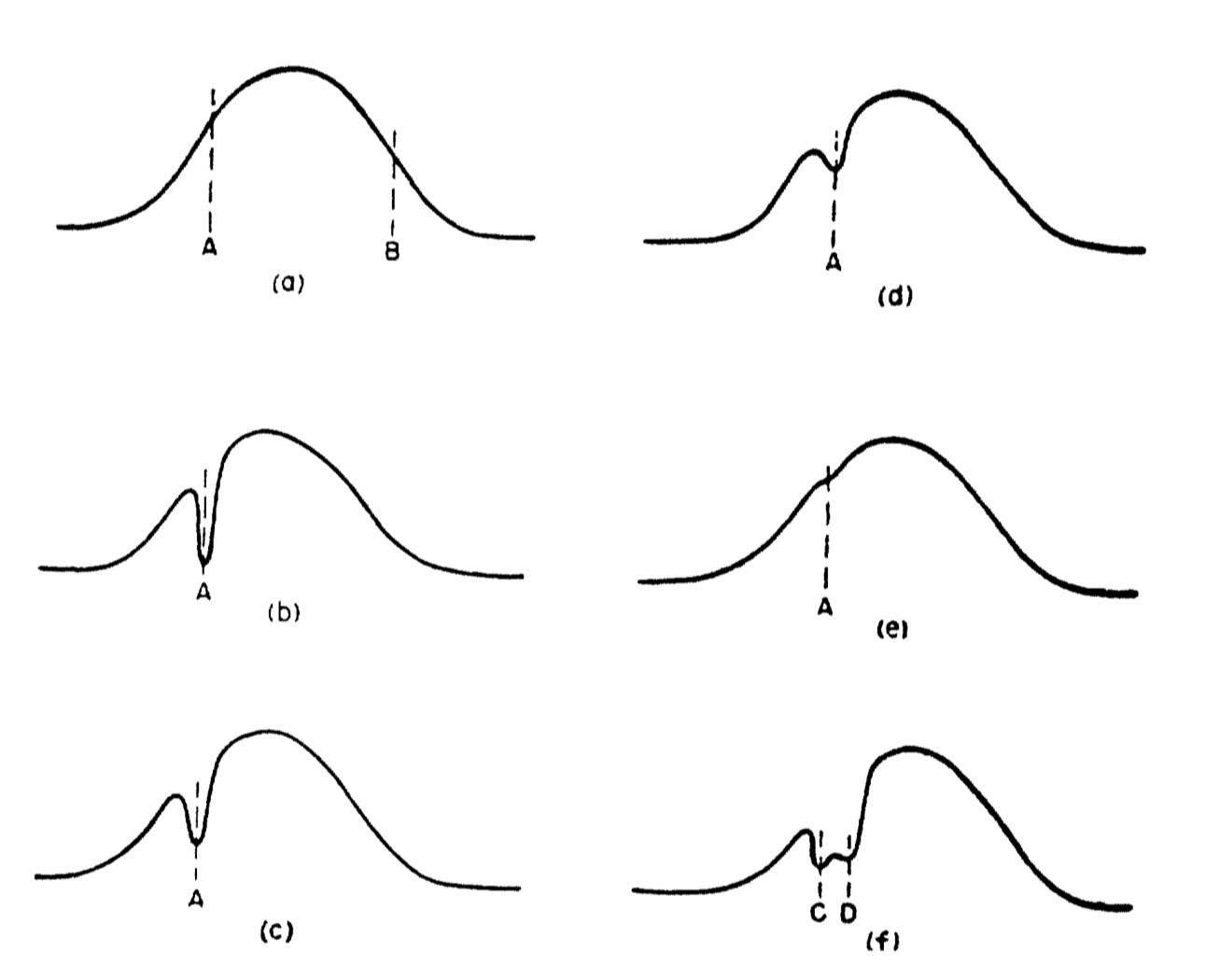
The earliest example of what could be called MRI in hind-sight is in the famous 1948 ‘BPP’ paper by Bloembergen, Purcell and Pound (Fig. 1)¹. The signals are from a water sample in an NMR spectrometer in the presence of gradient. The experiment was done before the advent of pulse Fourier transform (FT) NMR. The signal was recorded by sweeping the magnetic field through the ¹H resonance (called continuous wave or CW NMR), to yield directly, what appears to be a 1D projection of the cylindrical tube in the presence of a linear gradient (a). The paper says:
“the true width of the water resonance line was much less than the width…caused entirely by inhomogeneity of the field… With the field H0 maintained at a value corresponding to the point A… the absorption observed at A was caused by nuclei in one small part of the sample, that at B by those in another part. …the former group was subject to radiation at its resonance frequency all the time and was more or less thoroughly saturated…the gash in the curve betrays, quite literally, a hot spot (in respect to nuclear spin temperature) somewhere in the sample”.
Although the observation inspired no follow-up, it is the first example of the use of gradients and spatially selective excitation.
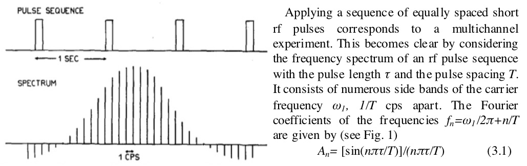
In 1966, Ernst and Anderson introduced the pulse FT method of NMR for high resolution spectroscopy applications (Fig. 2)². Instead of sweeping the field through the resonance(s), discrete pulses of RF at the NMR frequency were applied. The pulses excited a frequency bandwidth that is inversely proportional to the pulse duration. In the example provided, square RF pulses excited a bandwidth whose profile was a sinc (sinx/x) function. Over a decade later and conversely, sinc profile pulses would be used to excite square-profile bandwidths for slice-selection in the presence of linear magnetic field gradients. While not MRI per se, the use of pulses and a pulse sequence vs. field-sweep (CW) NMR is the back-bone of modern MRI methodology.
In 1971, Damadian reported that the NMR relaxation times of cancerous tissue were elevated compared to those of normal tissue³. Although this paper also does not mention imaging nor spatial localization, many of the early MRI papers that followed, referred to this work as evidence that if the NMR signal from normal and disease tissue differed, noninvasively imaging it with MRI, could have medical value. This provided a rationale for advancing the technology.
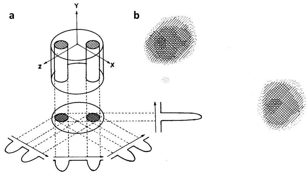
MRI began in earnest with Lauterbur’s 1973 Nature paper in which he presented a 2D image of two 1 mm tubes of water (Fig. 3)⁴. He reconstructed his image using the same back-projection method that had revolutionized X-ray computed tomography (CT). Even so, Lauterbur’s projections were not obtained by Ernst’s pulse FT method introduced 7 years earlier. Instead, the old BPP CW NMR method was used, along with the first-order linear shim gradient as the localization gradient on his 60 MHz NMR spectrometer. Lauterbur did not have the means to rotate this gradient in order to generate the angular projections, so he rotated the sample instead. At this time there was still no MRI pulse sequence or any slice selection.
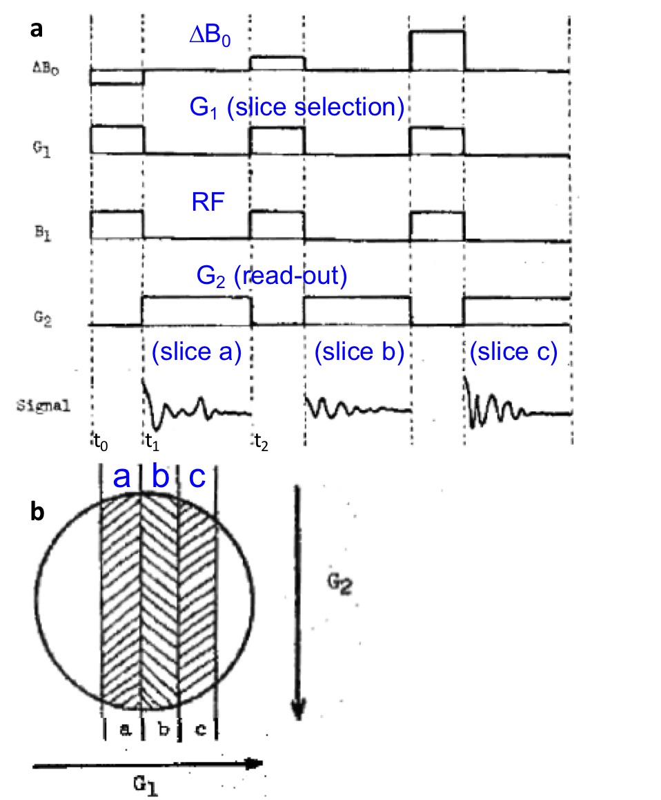
Lauterbur et al introduced slice selection at an NMR meeting at Nottingham in September 1974 (Fig.4)⁵. Here we see a pulsed FT method being applied and a first illustration of an MRI pulse sequence. A slice was selected by applying RF (B₁) in the presence of gradient G₁, followed by a readout gradient, G₂ to provide 1D projections. However, the slice was moved, not by shifting the RF frequency, but by offsetting the main field by ∆B_0, a reflection of the limited NMR spectrometers of the time. The gradients have no negative or oppositely-directed refocusing lobes, and the RF pulses are square (modulation was not possible). The latter meant, that even if the selective excitation pulses worked, they could only excite sinc-profile slices. The lack of negative lobes on the read-out gradient also did not account for the practicalities of turning the gradients on and off. Specifically, the first data points following excitation must be acquired because they sample the largest, lowest spatial-frequency components of the image according to the FT method. However, this is the period when the gradients are turned-on and are transient which causes huge low spatial-frequency image artefacts, ghosting etc.
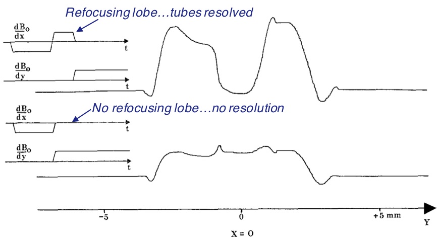
The missing gradient refocusing lobe on the selective excitation pulses was remedied by Hoult in 1977⁶. He argued that leaving them out would violate the Uncertainty Principle. Fig 5 shows his results, with and without the refocusing lobe. Without the refocusing lobe, spatial localization is essentially non-existent. This work introduced the ‘gradient-refocused echo’ (GRE) for MRI. However, the addition of the refocusing lobe after the RF excitation meant that the start of the read-out gradient had to be delayed. During this delay, signal was lost due to dephasing that was not recoverable when the projection was finally acquired.
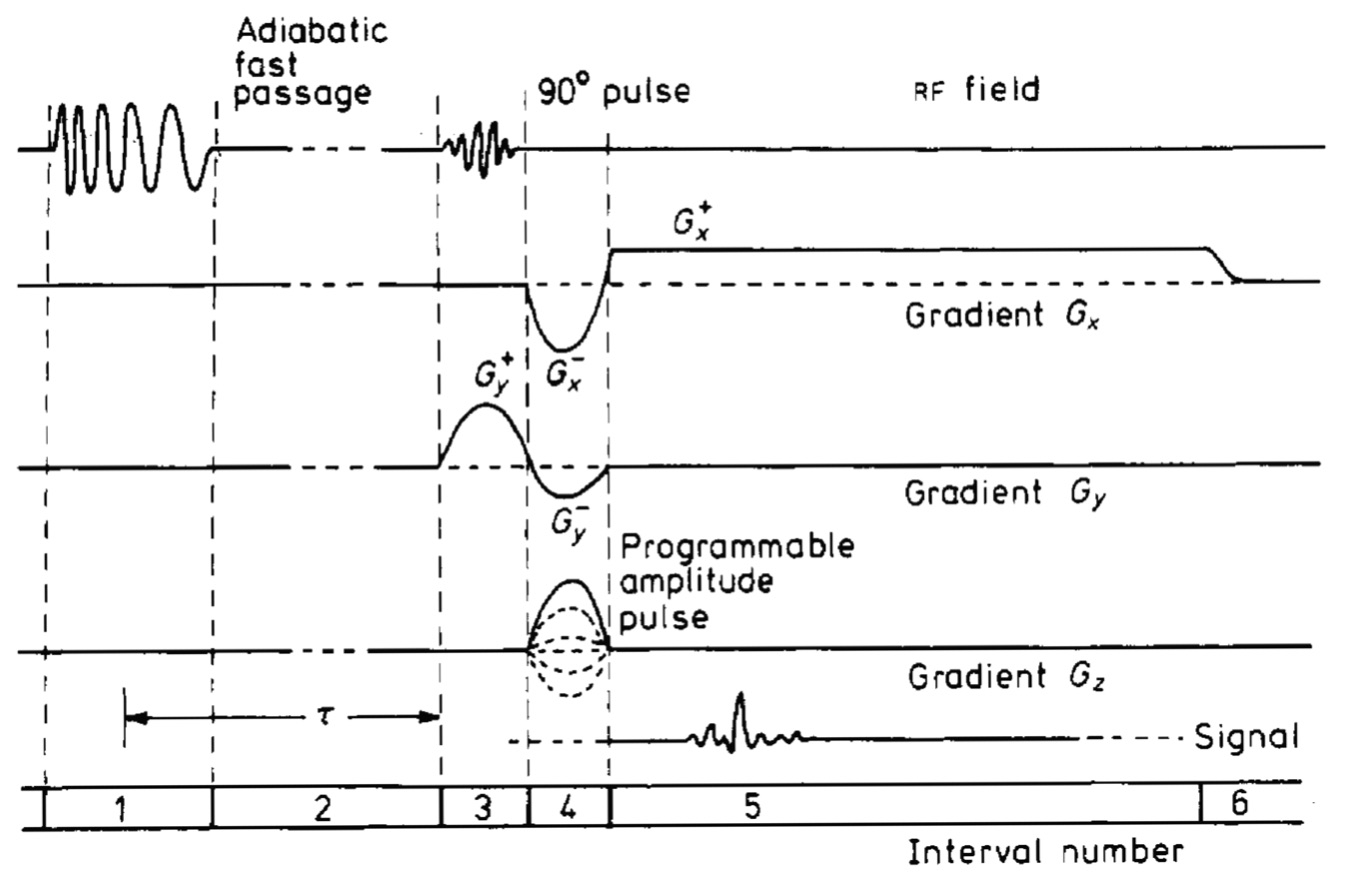
This problem and more, were fixed in the ‘spin warp’ method introduced by Edelstein et al in 1980 (Fig 6)⁷. In interval 3 we see the introduction of amplitude modulated RF pulses for selective excitation, manifest by a Gaussian-shaped RF pulse which excited a Gaussian profiled slice, instead of the bleeding sinc-profile. We see Hoult’s refocusing lobe on the (y) slice selective pulse in interval 4. Especially notable as well in interval 4, is the introduction of a new phase-encoding gradient (G_z). Indeed this paper introduced the spin-warp method that encodes the signal in the second, z-dimension, of the slice, replacing Lauterbur’s multiple angular projections. The read-out gradient, G_x in interval 5 generates a 1D projection in the x-direction. Importantly, a negative pre-lobe was also added to G_x in interval 4, to produce the GRE from signal originating along the x-direction to coincide with the GRE signal from the slice selection gradient (G_y here). By refocusing this signal to a time when the gradient is constant, the low spatial frequency components of the image are acquired without distortions from the switching-on of the gradients. Also here, an adiabatic fast passage (AFP) inversion pulse is added in interval 1 to allow T₁ measurements and/or T₁-weighted MRI.
While this scheme worked amazingly well on the Aberdeen group’s low B₀ = 0.04 T whole-body resistive magnet system, scaling it up, even just to 0.1 T resistive systems was untenable due to the effects of B₀ inhomogeneity in the magnets of that era. To overcome this, a 180° pulse was initially added to the Fig 6 sequence to generate a Carr-Purcell spin-echo, and the read-out gradient delayed until after the 180° pulse. However, this did not work either, due to the asymmetric dephasing effect of the read-out gradient on the refocusing signal. This problem was fixed by adding another gradient lobe before the 180° pulse. The amplitude and/or duration of the new lobe were adjusted to make the echo coincide with the true (T₂) spin-echo at time TE⁸, thereby overcoming residual magnet inhomogeneities. It also permitted T₂ and T₂-weighted MRI.
Other contributions to the development of MRI from the 1970s that have survived the decades since, include steady-state-free precession (SSFP a for-runner of FISP), which recognized early-on, the need to generate a continuous string of NMR signals to maximize spatial-encoding efficiency and the signal-to-noise ratio (SNR). This was used to acquire first 3D-resolved images of the human wrist at 500 projections/sec in 1977⁹. In 1982 Mansfield et al introduced echo-planar imaging (EPI), demonstrating the potential for cine imaging within the cardiac cycle in rabbits¹⁰.
These advances illustrate the evolution of MRI from an NMR experiment that was a curiosity showing that signals could be spatially selected in a simple field-sweep experiment in 1948¹, to the idea of NMR imaging inspired by X-ray CT³, to its reduction-to-practice in a modern-day looking MRI sequence⁷. Moreover, they illustrate the development of a whole new methodology wherein NMR signals are manipulated in space and time by adding and adjusting RF excitation and gradient pulses–their modulation, amplitudes and timing. These were the new building blocks for engineering desired MRI responses.

…Reduction-to-practice? That's not the whole story. Another key part of the show without which MRI would not exist today, is the massive engineering or applied physics effort and many inventions that were needed to build first, a working whole body scanner that could produce clinically useful images; and second, transform the technology to a product that could be used reliably and efficiently on patients in every day clinical settings.
The first set of heroes here, and they are quite unsung, are the magnet makers, who basically had to throw away Lauterbur-era NMR spectrometers that could only accommodate two 1mm tubes of water⁴, say; and up-regulate to systems with the ~1 m bore needed to accommodate the human body, transmit and receive coils, and 3 sets of gradient coils. The magnets had to be superconducting as well, at least in the beginning. This, in order to provide a sufficiently high B₀ to generate clinical images with the SNR, spatial resolution and efficiency, that could add real clinical value in medical imaging settings that already had X-ray, CT, ultrasound and nuclear imaging systems. In this context, MRI had to add value.
Whole-body superconducting magnet technology for MRI was pioneered by Oxford Instruments in England in the late 1970s and early 1980s. Field-strength was initially limited to 1.5 T¹¹ by the ability to manufacture the many km of continuous super-conducting wire required for the job. While B₀ for human-sized scanners has increased many-fold over the interim decades, 1.5T systems remain the most common workhorses for clinical MRI, to this day.
MRI gradient coil technology is another key contributor to MRI’s success. First there was distributed current “thumbprint” MRI gradients coils¹². Before these came along, one could only image out to 50-60% of the radius of the gradient coil due to aliasing and distortion. This meant that the magnets had to be even bigger to accommodate the gradient coils, not to mention their excessive power requirements due to their size. The thumb-print coils were further advanced by adding outer “self-shielding” coils, also a “thumbprint" design, to cancel out the gradient fields arising from eddy-currents induced by the inner gradient coils¹³. Without this technology, localized magnetic resonance spectroscopy (MRS), diffusion MRI including fiber track mapping, and many other techniques would not be possible today.
Then of course there was the RF coil technology. First came the bird-cage coil which basically made ≥1.5T MRI possible¹⁴. While surface NMR coils had been around since the 1970s, phased-arrays of them introduced in 1990¹⁵ not only afforded the maximum possible SNR, but also provided a means of accelerating the spatial encoding process, by using the coil’s inherently non-uniform individual sensitivity profiles^16,17.
…The 3rd leg of the stool on which MRI sits, is of course all of the clinical applications work, without which there would also be no clinical MRI. This is beyond the scope of this brief selection of what the author considers are key steps that have survived from the early development of MRI technology. This account is, inevitably, incomplete, as the time is indeed limited. For an expanded more-inclusive account of the story of MRI you might consider turning to the last reference in the list below¹⁸.

Acknowledgements

Support: None.