5198
3D CNN for Oxygen Extraction Fraction Mapping with combined QSM and qBOLD1Computer Assisted Clinical Medicine, Medical Faculty Mannheim, Heidelberg University, Mannheim, Germany
Synopsis
Keywords: Machine Learning/Artificial Intelligence, Oxygenation
We developed a CNN for OEF mapping from QSM+qBOLD data, which utilizes utilizes 3D convolutional layers. Two dimensions for the spatial components of an image and one dimension for the temporal component in the qBOLD data. The results are an improvement over our previous 2D CNN, but even the more advanced network architecture struggles with voxels, that have a very low deoxyhemoglobin content. In this abstract we also study with simulated data when the CNN produces reliable results and when it predicts default values for the reconstructed parameters instead.Introduction
The oxygen extraction fraction (OEF) can be used as an indicator for the vitality of tissue in pathologies that affect the blood perfusion like a stroke1 or that affect the tissues metabolism like cancer2. To determine the OEF we use a model that combines quantitative BOLD (qBOLD) and quantitative susceptibility mapping (QSM)3.Traditional fitting methods take a long time to reconstruct the parameter maps for a whole brain and strongly depend on the initial guess. Convolutional Neural Networks (CNNs) provide a way to get fast results without any initial guess. Previous works4 showed a lot of potential, so we worked on further improving the neural networks.
Methods
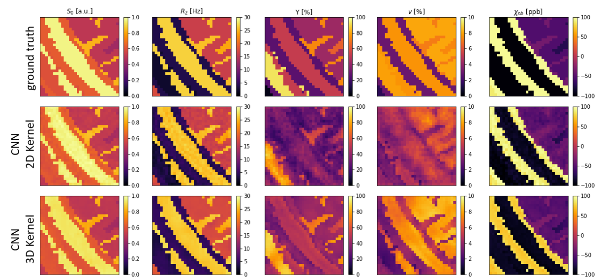
Artificial training data was created assuming the equations from the QSM+qBOLD model. It has 5 parameters: Initial signal amplitude S0, transverse relaxation rate R2, venous blood oxygenation Y, volume percentage of a voxel filled by deoxygenated blood ν and susceptibility χnb of the non-blood tissue surrounding the blood vessels. Y of the venous blood is used instead of OEF since OEF=(Ya -Yv )/Ya and Ya is assumed to be constant.To create training data patches of 30*30 pixels were taken from a segmented brain5. Random values for the 5 parameters were assigned to each tissue type in a patch. Example parameter maps can be seen in the top row of figure 1. The simulated signal was calculated for a GESFIDE sequence6 with a Spin Echo at 40 ms and 16 Gradient echoes spaced every 3 ms. Gaussian noise was added to the resulting signal to achieve an SNR of 100. The parameter maps were also used to calculate a quantitative susceptibility map of each patch, which is used as an additional input. The training set consists of approximately 200,000 patches.
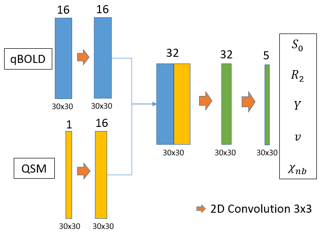
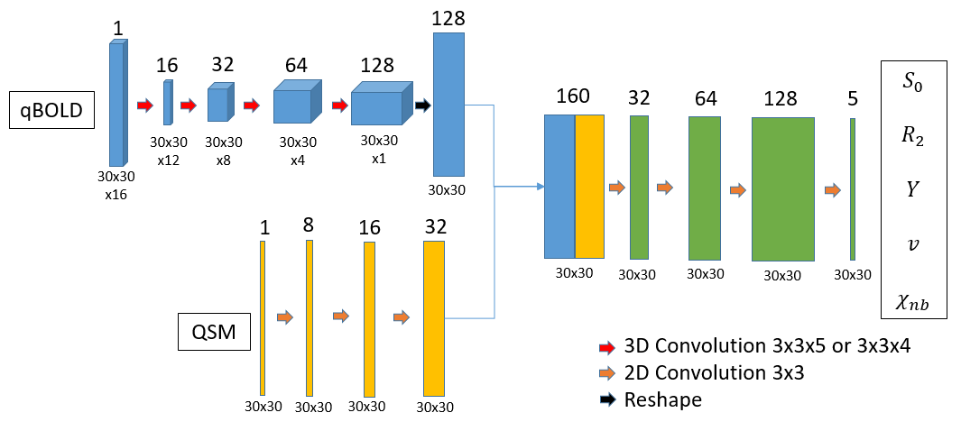
To reconstruct the parameters a simple CNN as shown and described in figure 2 was used in our previous work7. Figure 3 shows an improved CNN which utilizes 3D convolutions and has added batch normalization and spatial dropout. Both were implemented using Keras8 and TensorFlow9.
Results
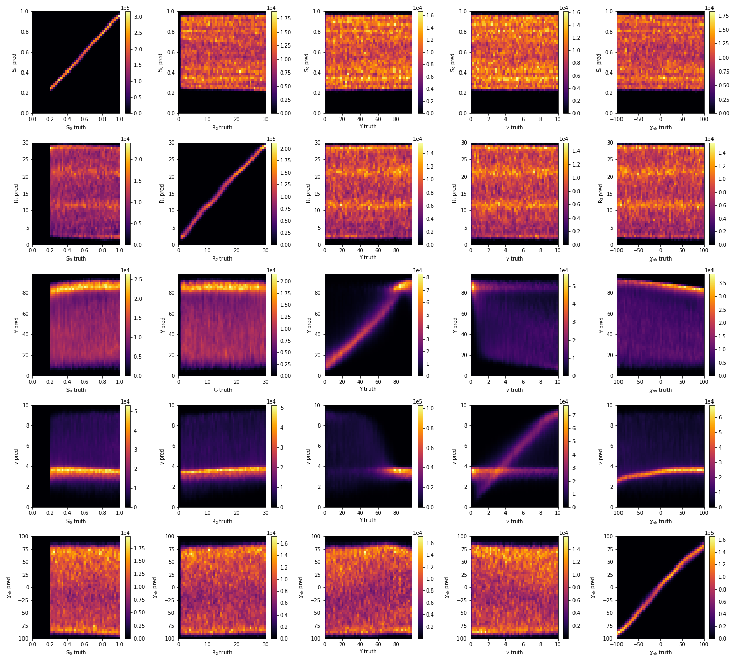
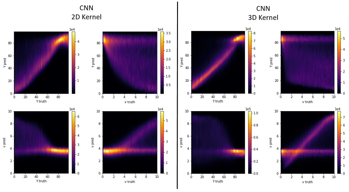
Figure 1 depicts the ground truth parameter maps of an exemplary patch together with the reconstruction results of both networks. The improved CNN with 3D convolutional layers leads to qualitatively better results for Y and ν, while it maintains a high level of accuracy for the other 3 parameters.Figure 4 gives an overview over the reconstruction accuracy of the CNN with 3D convolutions. Each subplot is a 2D histogram of all the true parameter values on the x axis vs the predicted parameter values on the y axis. A perfect result would be a thin line at an 45° angle for the subplots on the main diagonal and uniform noise for all other combinations. S0, R2 and χnb come close to the ideal, while Y and ν show clear correlations between them. These are further observed in figure 5, where the correlation plots of the CNN with 2D kernels is compared with the CNN with 3D kernels. Both networks show similar tendencies in parameter ranges with low deoxyhemoglobin content in a voxel. In these cases the additional signal loss from the deoxyhemoglobin is very small and the networks do not have enough information to accurately estimate the true values of Y and ν. The CNN with 3D kernels can still accurately predict Y down to ν of almost 2%. At ν below 2% it uses a default value for Y near 85%. Similar behavior is visible for predictions of ν when Y goes above 70%. Interestingly, both networks started to use the same default values of Y=85% and ν=3.5%. The older network never predicted a ν below 3% while the 3D CNN can go down to 1% for strongly deoxygenated blood with Y below 40%.
Discussion and Conclusion
The improved CNN with 3D convolutional layers can extract more information from the signal and has accurate predictions for a wider range of parameters. Other studies10 found strongly deoxygenated blood with an mean OEF around 50% and mean deoxygenated blood volume ν of 1%. The expected values for Y fall in the stable range of the networks, but the expected values for ν are below the possible range of the 2D CNN and at the edge of the range for the improved 3D CNN. Further improvements of the network architecture might move the range a bit more to lower values. To solve the problem we will continue by studying other sequences with more data points or higher SNR. Training a CNN with the same architecture as the 3D CNN on simulated data for possible sequences will provide a way to compare which sequences provide the most useful information.Acknowledgements
No acknowledgement found.References
1. Ibaraki M, Shimosegawa E, Miura S, Takahashi K, Ito H, Kanno I, Hatazawa J. PET measurements of CBF, OEF, and CMRO2 without arterial sampling inhyperacute ischemic stroke: method and error analysis. Ann Nucl Med 2004;18(1):35-44.
2. Vaupel P, Mayer A. Hypoxia in cancer: significance and impact on clinical outcome. Cancer Metastasis Rev 2007;26(2):225-239.
3. Hubertus, S, Thomas, S, Cho, J, Zhang, S, Wang, Y, Schad, LR. Comparison of gradient echo and gradient echo sampling of spin echo sequence for thequantification of the oxygen extraction fraction from a combined quantitative susceptibility mapping and quantitative BOLD (QSM+qBOLD) approach. MagnReson Med 2019;82:1491-1503.
4. Hubertus, S, Thomas, S, Cho, J, Zhang, S, Wang, Y, Schad, LR. Using an artificial neural network for fast mapping of the oxygen extraction fractionwith combined QSM and quantitative BOLD. Magn Reson Med. 2019; 82: 2199– 2211
5. Alfano, B, Comerci, M, Larobina, M, Prinster, A, Hornak, JP, Selvan, SE, Amato, U, Quarantelli, M, Tedeschi, G, Brunetti, A, Salvatore, M. An MRI digitalbrain phantom for validation of segmentation methods. Med Image Anal. 2011 Jun;15(3):329-39
6. Ma, J, Wehrli, F. Method for Image-Based Measurement of the Reversible and Irreversible Contribution to the Transverse-Relaxation Rate. J. Magn.Reson. B 1996; 111:61
7. Kinz, P, Schad, LR, A CNN for Oxygen Extraction Fraction Mapping with combined QSM and qBOLD, ISMRM 2022, Abstract 1986
8. Chollet, F et al, Keras, https://keras.io, 2015
9. Abadi, M et al, TensorFlow: Large-scale machine learning on heterogeneous systems, 2015. Software available from tensorflow.org.
10. Xiang, H, Yablonskiy, DA, Quantitative BOLD: Mapping of Human CerebralDeoxygenated Blood Volume and Oxygen ExtractionFraction: Default State, MagnReson Med 2007;57:115-126.
Figures