5188
Comparison of activation functions for optimizing deep learning models solving QSM-based dipole inversion1University Hospital Halle (Saale), Halle (Saale), Germany
Synopsis
Keywords: Machine Learning/Artificial Intelligence, Quantitative Susceptibility mapping
Deploying deep learning models for quantitative susceptibility mapping is driven by optimizing hyper-parameters and using suitable architectures. We investigated the impact of activation functions on network model training. ELU-, leaky ReLU- and ReLU-models with 16 and 32 initial channels were tested for solving dipole inversion on synthetic susceptibility data. All models showed convergence after completing 100 training epochs. However, the 16-channel-ELU-model achieved low losses after only 20 training epochs and showed similar reconstruction performance to the 32-channel-ELU-model. Using the ELU activation allows the use of smaller network models resulting in fewer memory requirements and less training time.Introduction
Convolutional neural networks (CNNs) are widely used for image analysis and, in recent years, for solving dipole inversion of quantitative susceptibility mapping (QSM)1. The activation functions of neural networks are non-linear transformations performed over the weighted sum of the input signal producing the output of nodes in network layers. Selecting the appropriate activation function is similarly crucial for accelerating network training and obtaining generalizable network models as the choice of appropriate hyper-parameters. Therefore, we provide comprehensive and systematic analysis of three commonly used activation functions for training the U-Net2 for solving the field-to-susceptibility problem of QSM on synthetic data.Methods
A standard U-Net2, receiving synthetic 3D input data was trained to predict the 3D susceptibility map from the same-sized input magnetic field distribution. The network architecture of all models was five layers deep with 16 or 32 initial channels (IC). Three different activation functions, ReLU3, leaky ReLU4 (α=-0.2, like QSMGAN5) and ELU6 (α=1, default parameter) were used during training (Fig. 1). 1000 synthetic non-anatomical susceptibility maps (320x320x320) compromising randomly distributed spheres and rectangles with susceptibilities from a Gaussian distribution (µ=0, σ=0.25) and Gaussian smoothing applied to each shape individually served as training data. Image border regions (at least 40 voxels) of susceptibility maps were set to zero by randomly inserting ellipsoids of different extension. The B-field distribution was obtained by fast forward convolution in k-space7. Four patches (160x160x160) were randomly extracted from these datasets at each iteration for training. The models were trained using the AdamW8 optimizer for 100 epochs with a learning rate of 0.001 and weight decay of 0.01. Physics-informed training was performed on an NVIDIA A100 GPU. The loss measures the similarity of the susceptibilities and enforces data regularization via the physical model (λ=1) by comparing the B-field distributions (Fig. 2D). Validation was performed after completion of each epoch on 100 validation datasets. The network models were evaluated on synthetic data corresponding to the training dataset to increase comparability of results and assessment.Results
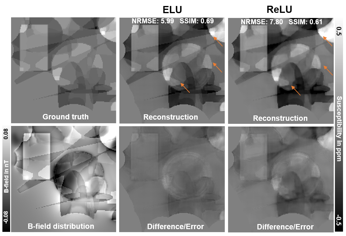
While the convergence of loss measures for the different models develops similarly on the training set (Fig. 2A), substantial differences are visible on validation data (Fig. 2B and 2C). Here, the 16-IC-ELU-model reaches low loss and mean NRMSE values at early epochs. The 16-IC-models with ReLU or leaky ReLU activation show a different convergence, leading to almost twice as high loss values and leaving a gap to the other models. Similar metrics are obtained by all 32-IC-models after completion of 100 epochs of training. The evaluation on synthetic test data (Fig. 3) shows that the differences between the models after 100 training epochs are in subtleties (orange arrows) like sharp edges or tiny structures. Based on NRMSE, SSIM and visual assessment, the ELU-model achieves greatest similarity with the ground truth and least remnants in the difference map. Since the ELU-model with 16 IC showed low loss values at early epochs, two 16-IC-models with ELU and ReLU activation were evaluated after training for 20 epochs (Fig. 4). The NRMSE and SSIM values together with the visual assessment show higher similarity of the ELU-model compared with the ground truth as the ReLU-model. The susceptibility map of the ELU model shows more details and sharper edges.Discussion
Sparsity is introduced into ReLU-networks via the dying-ReLU-problem leading to a substantial amount of network nodes not contributing to the computations. While the 16-IC-model lacks fast parameter convergence and low metrics, the opposite can be seen for the 32-IC-model. Thus, for the 16-IC-model, sparsity is an issue, while for the 32-IC-model, the strength of sparsity is that not all nodes contribute to the computation and therefore fewer parameters need to be optimized. The ELU activation function eliminates the dying-ReLU problem leading to all nodes contributing to the final computation. Furthermore, ELU allows negative values, pushing the mean of activations closer to zero and enabling faster learning by bringing the gradients closer to the natural gradients therewith6. Hence, the 16-channel ELU-model exhibits fast convergence and low loss values at early epochs. Consequently, choosing the ELU activation allows the use of a smaller CNN with 16 IC, accelerating network training and reducing memory requirements. The 32-IC-ELU-model shows similar results after 100 training epochs. Thus, ELU-models can compensate for their higher memory and training requirements by allowing the use of smaller models. Hence, building smaller models by choosing ELU activation enables training and inference on smaller GPUs. The differences between leaky ReLU-models and ELU-models can be explained by the saturation plateau introduced with ELU, allowing ELU-models to learn more stable representations6. Different parameters for activation functions are subject of further investigations. Remaining differences between reconstructed and ground truth susceptibilities can be reduced with more training epochs. The findings of this abstract may be applicable to different topics like image segmentation/classification and thus, smaller models using ELU activation might be possible as well.Conclusion
This work underlines the importance of selecting an appropriate activation function. Using the ELU activation leads to fast convergence with the ELU-models outperforming its opponents. The ELU activation enables the deployment of smaller network models that reduce the memory requirements and training time.Acknowledgements
This project was supported by the European Regional Fund (ERDF - IP* 1b, ZS/2021/06/158189).References
- Yoon J, Gong E, Chatnuntawech I. (2018). Quantitative susceptibility mapping using deep neural network: QSMnet. Neuroimage. https://doi.org/10.1016/j.neuroimage.2018.06.030
- Ronneberger O, Fischer P, Brox T. (2015). U-Net: Convolutional Networks for Biomedical Image Segmentation. Medical Image Computing and Computer-Assisted Intervention – MICCAI 2015. https://doi.org/10.1007/978-3-319-24574-4_28
- Nair V, Hinton GE. (2010). Rectified linear units improve restricted boltzmann machines. Proceedings of the 27th International Conference on International Conference on Machine Learning (ICML)
- Maas AL, Hannun AY, Ng AY. (2013). Rectifier Nonlinearities Improve Neural Network Acoustic Models. Proceedings of the 30th International Conference on Machine Learning (ICML)
- Chen Y, Jakary A, Avadiappan S et al. (2020). Improved Quantitative Susceptibility Mapping using 3D Generative Adversarial Networks with increased receptive field. Neuroimage. https://doi.org/10.1016/j.neuroimage.2019.116389
- Clevert DA, Unterthiner T, Hochreiter S. (2015). Fast and Accurate Deep Network Learning by Exponential Linear Units (ELUs). https://doi.org/10.48550/arxiv.1511.07289
- Marques P, Bowtell R. (2005). Application of a Fourier‐based method for rapid calculation of field inhomogeneity due to spatial variation of magnetic susceptibility. https://doi.org/10.1002/cmr.b.20034
- Loshchilov I, Hutter F. (2017). Decoupled Weight Decay Regularization. https://doi.org/10.48550/arxiv.1711.05101
Figures
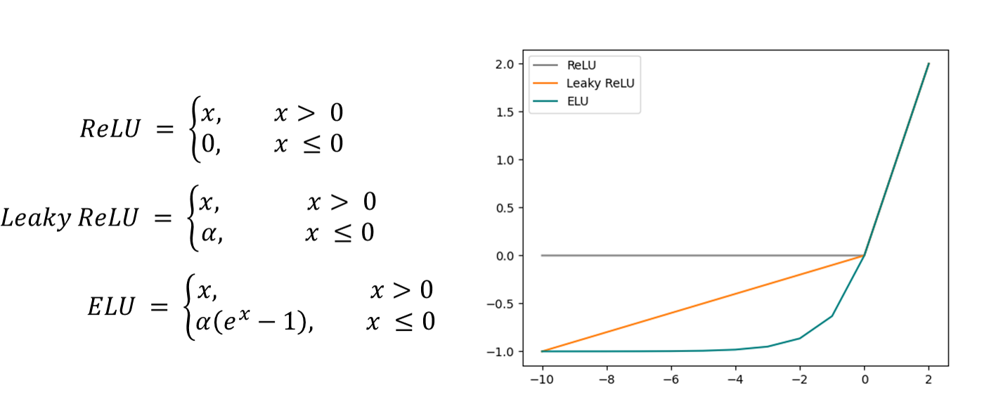
Figure 1: Equations of the ReLU, leaky ReLU and ELU activation function together with a plot of these functions. The activation functions are identical for positive x values but show different characteristics for negative x-values. ReLU is zero for negative values. The leaky ReLU and ELU are characterized by a linear or exponential increase in the negative regime.
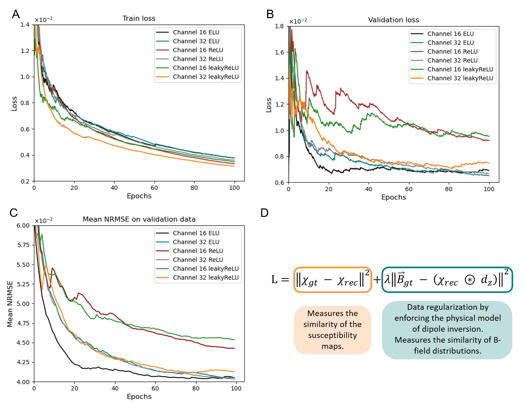
Figure 2: Development of loss measures on the train (A) and validation set (B) and the mean NRMSE (C) of the models compared to the ground truth trained with the ELU, leaky ReLU and ReLU activation function and 16 or 32 initial channels. The loss function (D) is used for parameter updates during training (λ=1). dz is the z-component of the point dipole response. The 16 channel ELU-model shows fastest convergence on validation data and scores low metrics after completing 20 training epochs.
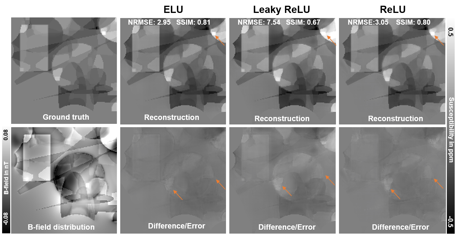
Figure 3: Comparison of reconstructed susceptibility maps and difference maps of ELU-, leaky ReLU- and ReLU-models with 32 initial channels after completing 100 training epochs. Orange arrows indicate a tiny structure in the susceptibility map and edge remnants in the difference. NRMSE (lower is better) and SSIM (higher is better) were computed over the entire dataset. All reconstructed maps resemble the ground truth with differences being present in sharp edges, tiny structures and metrics.