5181
Training Strategies for Convolutional Neural Networks in Prostate T2 Relaxometry
Patrick Bolan1, Sara Saunders1, Mitchell Gross1, Kendrick Kay1, Mehmet Akcakaya2, and Gregory Metzger1
1Center for MR Research / Radiology, University of Minnesota, Minneapolis, MN, United States, 2Electrical and Computer Engineering, University of Minnesota, Minneapolis, MN, United States
1Center for MR Research / Radiology, University of Minnesota, Minneapolis, MN, United States, 2Electrical and Computer Engineering, University of Minnesota, Minneapolis, MN, United States
Synopsis
Keywords: Machine Learning/Artificial Intelligence, Prostate, Relaxometry
This work uses convolutional neural networks (CNNS) with two training strategies for estimating quantitative T2 values from prostate relaxometry measurements, and compares the results to conventional non-linear least squares fitting. The CNN trained with synthetic data in a supervised manner gave lower median errors and better noise robustness than either NLLS fitting or a CNN trained on in vivo data with a self-supervised loss.Introduction
Quantitative T2 mapping can provide valuable information for prostate cancer diagnosis. Relative to qualitative T2-weighted imaging, quantitative T2 maps give a more objective and potentially sensitive imaging biomarker for diagnosis and grading of prostate cancer (1–3). Mapping is generally performed by acquiring a series of images at multiple echo times, followed by non-linear least squares (NLLS) fitting on a pixel-by-pixel basis to estimate T2 (Figure 1). Prior work from relaxometry (4,5) and similar diffusion applications (6–9) has found that replacing the NLLS fitting with a trained neural network (NN) can greatly speed up processing (6) and reduce the bias associated with least-squares fitting of magnitude images, which have Rician noise (10,11).One difficulty with these NN approaches is how to perform the training with in vivo data, where the true T2 value is not known. In this work we implement convolutional neural networks (CNNs) trained with two distinct strategies and compare their performance with the conventional NLLS: a self-supervised training strategy, previously described for diffusion problems (6,8), and supervised training using a large synthetic dataset based on the ImageNET database of labelled photographs (12,13), a strategy previously used in image reconstruction (14). We trained CNNs using both strategies and compared their performance with NLLS in synthetic and in vivo datasets. Results showed that both CNNs outperformed NLLS in terms of absolute error, bias, and noise robustness.
Methods
Prostate MRI was acquired on a Siemens 3T Prisma scanner with surface and endorectal receive coils under an IRB-approved protocol. Multi-echo multi-slice fast spin-echo MR images were acquired from 118 participants using the vendor’s spin-echo multi-contrast sequence, with parameters TR=6000 ms, TE=13.2-145.2 ms in 11 increments, 256x256 images with resolution 1.1x1.1 mm, 19-28 slices 3 mm thick. The first echo was discarded to avoid stimulated echo artifacts. Images were split into 86 cases for training and 32 for independent testing.To generate a synthetic dataset, two sequential images from ImageNET were selected for S0 and T2, scaled (S0 Î[0,1] and T2 Î[0.6.5, 580] ms), and noise was added to create a multi-echo image series with Rician noise following S(TE) = |S0 * exp(-TE/T2) + N(0,σ2) +i N(0,σ2) |, where N(0,σ2) is a Gaussian distribution, with σ sampled from a uniform distribution over [0.001, 0.1]. Ten thousand image series were synthesized for training, and a separate 1,000 series for independent evaluation.
CNNs were based on the enhanced U-Net provided in the MONAI (15) library, with 10 input channels, 4 layers of widths [128, 128, 256, 512], 2 output channels, and 3x3 convolution kernels throughout. The CNN_IMAGENET model was trained in a supervised manner, with a mean squared error (MSE) loss relative to the ground truth S0 and T2. The CNN_SS_INVIVO model was trained using the in vivo training dataset by using the S0 and T2 values output from the network to simulate values of S(TE), and the MSE between simulated and measured data was used as a loss function. Both CNNs were trained in PyTorch (16) for 1000 epochs, batch size=100, AdamW optimizer, LR=0.002. The conventional fitting (FIT_NLLS) used optimize.curve_fit() from Scipy (17) to fit the data to a monoexponential curve to estimate S0 and T2.
Additionally, a noise-addition experiment was performed to evaluate the sensitivity of each method to progressively increasing Rician noise, added artificially to the in vivo evaluation dataset.
Results
Figure 2 gives an example case from the synthetic IMAGENET dataset. In the high-SNR regions the three methods produce similar-appearing results, although CNN_IMAGENET has lower noise. The estimated T2 maps are most different in the low-SNR regions, where the FIT_NLLS show high noise levels, whereas CNN_IMAGENET appears to show blurring.Figure 3 provides a quantitative comparison of the methods’ performance in estimating T2 maps on the synthetic dataset. In this comparison CNN_IMAGENET has the smallest error and smallest variability of error, and does not show the positive bias (T2pred > T2true) at low SNR seen with FIT_NLLS or CNN_SS_INVIVO.
An example comparing the three methods on an in vivo test case is given in Figure 4. The results appear similar in high SNR regions but differ in lower SNR areas, consistent with the findings on the synthetic test set. The CNN_IMAGENET again shows some evidence of blurring.
Figure 5 shows the impact of increasing noise levels. The noise in the source images propagates into the FIT_NLLS T2 map, but the CNN_IMAGENET map shows consistent results even at high noise levels. As in the synthetic dataset, the CNN_SS_INVIVO method exhibits a modest improvement over FIT_NLLS.
Discussion
The FIT_NLLS and CNN_SS_INVIVO methods showed bias at low SNR levels and sensitivity to increasing noise in the in vivo data, whereas CNN_IMAGENET gave improved accuracy at high noise levels. These results are attributable to CNN_IMAGENET’s ability to correctly model the Rician noise distribution, and the training strategy which provided implicit denoising. Downsides of this synthetic/supervised training strategy include blurring and potential sensitivity to the distribution of T2 values in the training dataset.Conclusion
We found that a CNN, trained with synthetic data in a supervised manner, gave lower median errors, and better noise robustness than either NLLS fitting or a CNN trained on with a self-supervised loss.Acknowledgements
This work was sponsored by NIH P41 EB027061, NIH R01 CA241159, NIH S10 OD017974-01References
1. Mai J, Abubrig M, Lehmann T, et al. T2 Mapping in Prostate Cancer: Invest. Radiol. 2019;54:146–152 doi: 10.1097/RLI.0000000000000520. 2. Klingebiel M, Schimmöller L, Weiland E, et al. Value of T 2 Mapping MRI for Prostate Cancer Detection and Classification. J. Magn. Reson. Imaging 2022;56:413–422 doi: 10.1002/jmri.28061. 3. Metzger GJ, Kalavagunta C, Spilseth B, et al. Detection of Prostate Cancer: Quantitative Multiparametric MR Imaging Models Developed Using Registered Correlative Histopathology. Radiology 2016;279:805–816 doi: 10.1148/radiol.2015151089. 4. Müller-Franzes G, Nolte T, Ciba M, et al. Fast, Accurate, and Robust T2 Mapping of Articular Cartilage by Neural Networks. Diagnostics 2022;12:688 doi: 10.3390/diagnostics12030688. 5. Saunders SL, Gross M, Metzger GJ, Bolan PJ. T2 Mapping of the Prostate with a Convolutional Neural Network. In: Proceedings 30th Scientific Meeting, ISMRM. London, UK; 2022. p. 3915. 6. Barbieri S, Gurney‐Champion OJ, Klaassen R, Thoeny HC. Deep learning how to fit an intravoxel incoherent motion model to diffusion‐weighted MRI. Magn. Reson. Med. 2020;83:312–321 doi: 10.1002/mrm.27910. 7. Bertleff M, Domsch S, Weingärtner S, et al. Diffusion parameter mapping with the combined intravoxel incoherent motion and kurtosis model using artificial neural networks at 3 T. NMR Biomed. 2017;30:e3833 doi: 10.1002/nbm.3833. 8. Kaandorp MPT, Barbieri S, Klaassen R, et al. Improved unsupervised physics‐informed deep learning for intravoxel incoherent motion modeling and evaluation in pancreatic cancer patients. Magn. Reson. Med. 2021;86:2250–2265 doi: 10.1002/mrm.28852. 9. Vasylechko SD, Warfield SK, Afacan O, Kurugol S. Self‐supervised IVIM DWI parameter estimation with a physics based forward model. Magn. Reson. Med. 2022;87:904–914 doi: 10.1002/mrm.28989. 10. Raya JG, Dietrich O, Horng A, Weber J, Reiser MF, Glaser C. T2 measurement in articular cartilage: Impact of the fitting method on accuracy and precision at low SNR. Magn. Reson. Med. 2009:NA-NA doi: 10.1002/mrm.22178. 11. Bouhrara M, Reiter DA, Celik H, et al. Incorporation of rician noise in the analysis of biexponential transverse relaxation in cartilage using a multiple gradient echo sequence at 3 and 7 tesla: Rician Noise and Analysis of Relaxation. Magn. Reson. Med. 2015;73:352–366 doi: 10.1002/mrm.25111. 12. Deng J, Dong W, Socher R, Li L-J, Li K, Fei-Fei L. ImageNet: A large-scale hierarchical image database. In: 2009 IEEE Conference on Computer Vision and Pattern Recognition. ; 2009. pp. 248–255. doi: 10.1109/CVPR.2009.5206848. 13. ILSVRC2012 Validation Set. https://www.kaggle.com/datasets/samfc10/ilsvrc2012-validation-set. Accessed November 4, 2022. 14. Zhu B, Liu JZ, Cauley SF, Rosen BR, Rosen MS. Image reconstruction by domain-transform manifold learning. Nature 2018;555:487–492 doi: 10.1038/nature25988. 15. The MONAI Consortium. Project MONAI. 2020 doi: 10.5281/zenodo.4323059. 16. Paszke A, Gross S, Massa F, et al. PyTorch: An Imperative Style, High-Performance Deep Learning Library. :12. 17. Virtanen P, Gommers R, Oliphant TE, et al. SciPy 1.0: fundamental algorithms for scientific computing in Python. Nat. Methods 2020;17:261–272 doi: 10.1038/s41592-019-0686-2.Figures
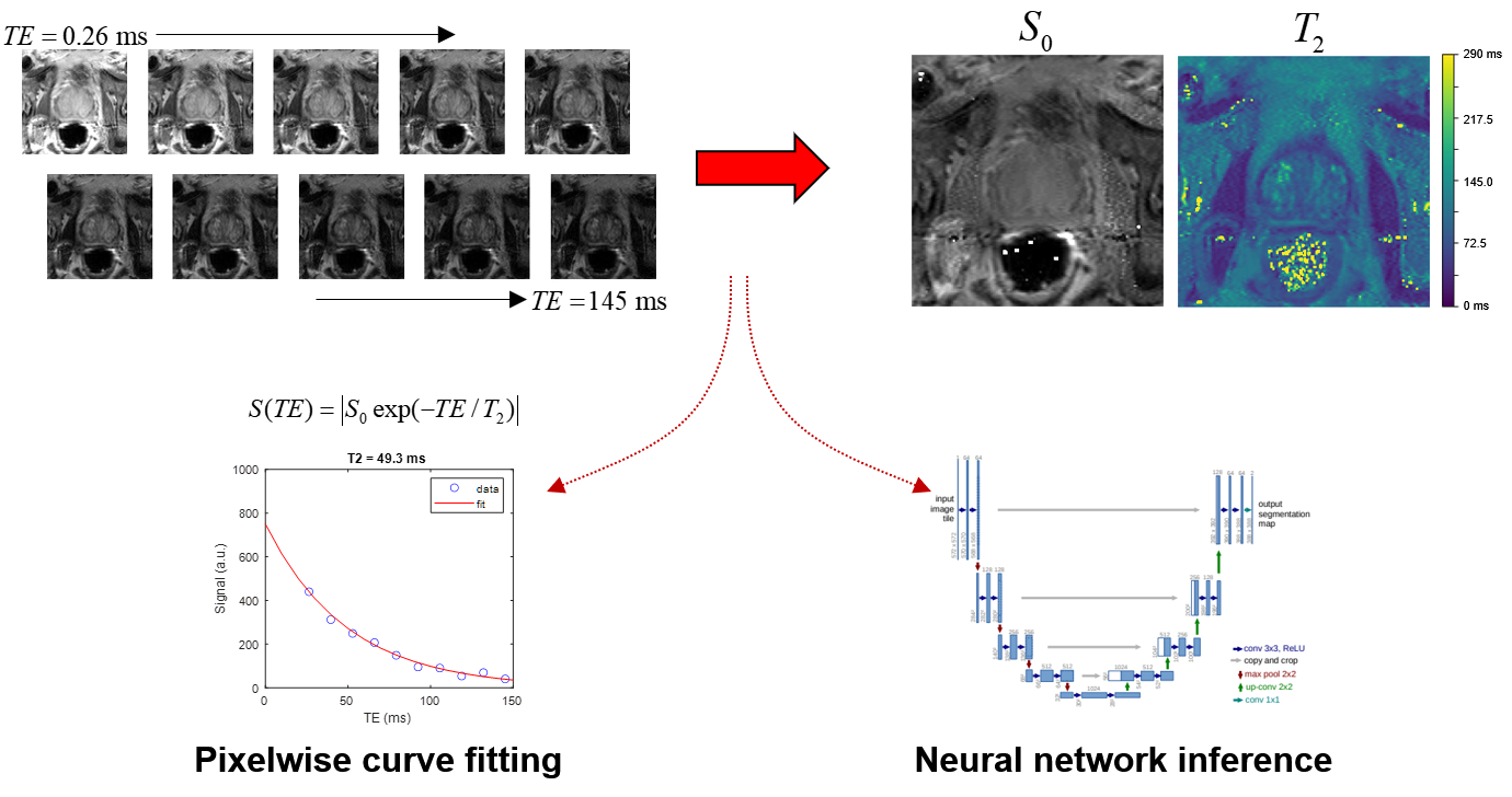
Overview of the prostate T2 relaxometry problem.
A series of spin-echo images are acquired at multiple echo times. The
conventional approach fits the TE series one pixel at a time to a mono-exponential
decay curve to produce maps of S0 and T2. Alternatively, a CNN can be trained
to take the image series as input and produce S0 and T2 maps as output.
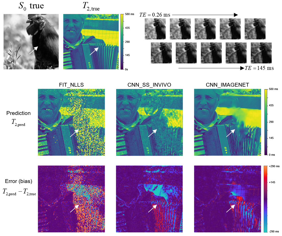
Example showing estimated T2 maps from all three
methods for a case from the synthetic IMAGENET test dataset, with the true S0
and T2 map shown above. The regions of low S0 values (e.g., white arrow) give
low SNR, which can be seen as regions of incorrect values in each of the
estimated T2 maps. This example shows how the methods vary in performance at
various noise levels and how they fail in regions of very low SNR.
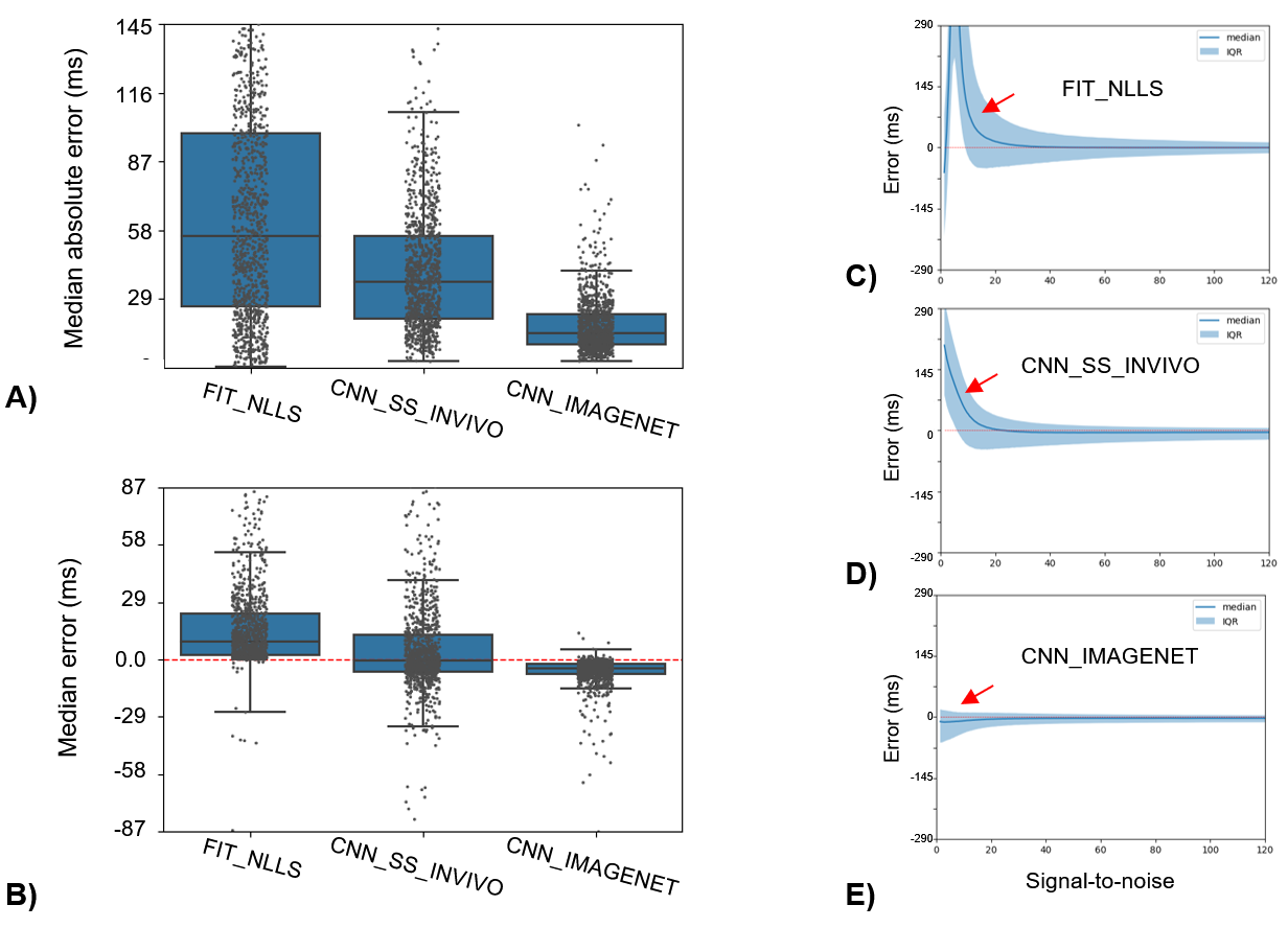
T2 estimation error (T2,pred-T2,true)
for the three methods evaluated in the IMAGNET test dataset. A) Median absolute
error, with box-whiskers showing median and interquartile ranges (IQR), shows
that CNN_IMAGENET has the lowest error and smallest variability. B) The signed
error can be interpreted as bias: FIT_NLLS has a positive bias, whereas CNN_IMAGNET
has small bias with minimal variation. C-E) Error and IQR evaluated on a
per-pixel basis as a function of SNR. Both FIT_NLLS and CNN_SS_INVIVO show T2 bias
at low SNR (red arrows) due to the Rician noise distribution.
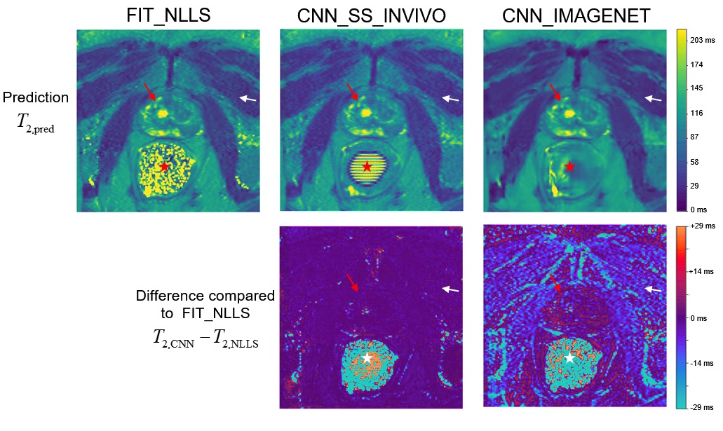
Comparison of parameter estimation methods on a
single example slice from the in vivo evaluation dataset. Since no true value
of T2 is available, the methods are compared to the standard FIT_NLLS.
The top row shows T2 maps from each method, with similar results in high-SNR
regions like the prostate (red arrows) but greater differences in the low-SNR muscle
region (white arrows). In the air-filled rectum (star) the true S0 is zero;
thus the resulting T2 values demonstrate how the methods fail differently in the
limit of low SNR.
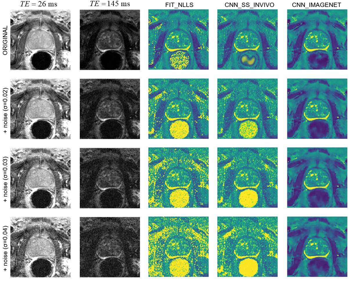
An example case from the noise-addition
experiment. The top row shows the unmodified data: images of the shortest and
longest echo time, and T2 maps calculated with the three selected estimation
methods. The next three rows show the same data with increasing noise added and
the corresponding T2 maps. With increasing noise, FIT_NLLS shows longer T2 values
and increased noise; CNN_SS_INVIVO is similar with moderately less noise,
CNN_IMAGENET shows only modest blurring.
DOI: https://doi.org/10.58530/2023/5181