5171
Fast consensus optimisation in diffusion MRI modeling
Samuel St-Jean1 and Markus Nilsson1
1Clinical Sciences Lund, Lund University, Lund, Sweden
1Clinical Sciences Lund, Lund University, Lund, Sweden
Synopsis
Keywords: Diffusion/other diffusion imaging techniques, Data Analysis, diffusion modeling
This work explores how to obtain parameter maps from a diffusion MRI model under 30 seconds and how to leverage multiple plausible solutions into a consensus solution using a framework similar to MR fingerprinting. The method is tested with a two compartments model and a mean kurtosis model and compared with a standard optimisation solver. Visual improvements are shown on parameter maps, showing less implausible values than the standard method, but without the use of constraints or assumptions. Access to a distribution of plausible values allows to compute most likely value from this distribution in the case of parameter degeneracies.Introduction
The everyday diffusion MRI (dMRI) acquisition is lengthy and requires additional processing before interpretation of a biophysical model of choice. The classical optimisation solution can also lead to multiple values that explain equally well the dMRI signal due to degeneracies in the optimisation landscape, leading to inaccurate parameter maps1. This work explores how to obtain parameter maps from a biophysical model covering the full brain under 30 seconds and how to leverage multiple plausible solutions into a consensus solution instead, allowing quantification of the variability of the solution. This approach instead relies on defining a valid biophysical model and an interval of values for its parameters and leverages a GPU for fast computations. No constraints simplifying the model are needed to stabilize the solution as they could be incorrect (e.g. in the presence of disease), but implausible signals are instead discarded upfront from the admissible candidate signals.Methods
Following the framework of MR fingerprinting2, the powder-averaged dMRI signal is matched against a database of candidate signals projected on the smallest spanning subspace of the diffusion model3,4,5. A first pass selects the top matching parameter values for each voxel. A second pass then calculates the best 500 matches to build a distribution of parameters for each voxel, using only the plausible candidates identified in the previous step to reduce the search space. This is beneficial as we do not have to restart the optimisation process from multiple initial guesses or assume that we found the only correct solution as in classical optimisation. Finally, aggregate values are computed to represent the distribution and its variability, such as the mean and coefficient of variation (CV, defined as the standard deviation over the mean). Two models were used to showcase the flexibility of the method. The first model (see Eq. 1) is a two compartments model with a stick compartment to capture the intra-axonal diffusivity and a zeppelin compartment to capture the extra-cellular diffusivity. The second model (see Eq. 2) is a kurtosis model with mean diffusivity D and mean kurtosis K as free parameters. As the method only needs to know how to generate the forward signal, any other model can be used at runtime without requiring additional tuning or optimisation besides choosing the range of plausible values. Here we chose to restrict the fractions to sum to 1 and limit the diffusivities between 0.1 um2/ms and 3 um2/ms in steps of 0.1 um2/ms to build the dictionary of the first model. In the kurtosis model, we use the same interval for D and restrict K between -2 and 15 in steps of 0.1. Values of K generating increasing signal for a given b-value or when $$$K>=3/(bD)$$$ were also excluded beforehand to prevent implausible cases6. We also benchmark the results against a classical L2 norm minimisation initialised at random from a uniform distribution for each voxels using the same bounds as the proposed method.$$\text{Eq.1}S_b/S_0=f_1\sqrt{\pi/4x_1}\text{erf}(\sqrt{x_1})+f_2\sqrt{\pi/4x_2}\exp(-bD_{par})\text{erf}(\sqrt{x_2})$$
where $$$x_1=bD_{par},x_2=b(D_{par}-D_{perp})$$$ and erf is the error function.
$$\text{Eq.2}\log(S_b/S_0)=-bD+1/6(bD)^2K$$
Datasets
We used a publicly available 3 shells dataset7 acquired on a 3T Philips scanner at 2mm isotropic, TR/TE=5615/95ms and SENSE=2 for a total acquisition time of 10 minutes. The dataset consists initially of 7x b=0, 8x b=0.3, 32x b=1 and 60x b=2 um2/ms volumes before averaging. The data was also motion corrected and corrected for eddy currents using FSL before averaging.Results
Figure 1 shows an example of a synthetic signal with the kurtosis model where both methods give similar results, with the proposed method being an order of magnitude faster. Figures 2 and 3 show an axial slice for each parameter of the studied models. The entire process takes around 20s on a standard laptop with an Nvidia 2080 GPU for a full brain dataset, which is approximately 50x faster than the classical optimisation algorithm. Noticeably, the spatial coherence of the parameter maps is improved over the classical optimisation without requiring strong parameter constraints or prior assumptions for both models. We surmise that this is because multiple plausible guesses are available at each voxel instead of a single value as in classical optimisation. In the case of multiple minima in the optimisation landscape, this might provide a viable alternative to only choosing the ‘optimal’ solution as a distribution of values can be summarised by choosing the mean, the mode or the median of the distribution.Discussion and Conclusion
We presented a fast optimisation method which computes distribution of plausible values under a minute, possibly indicating regions where the model or the acquisition scheme might be less reliable as suggested by a higher variability. An interesting use case would be researchers wanting to analyse thousands of datasets without needing a computing cluster as the only computational requirement is to possess a consumer grade GPU. Additionally, access to a distribution of plausible values allows researchers to estimate the uncertainty of their models and prevent relying on a single optimal value, which might be incorrect due to errors in the optimisation algorithm. This is especially useful as we can now compute a most likely value from this distribution in the case of parameter degeneracies – a case which is currently not covered by classical optimisation methods.Acknowledgements
No acknowledgement found.References
[1] Jelescu et al. 2015 NMR Biomedicine
[2] Ma et al. 2013 Nature
[3] Lasic et al. 2014 Frontiers in Physics
[4] McGivney et al. IEEE 2014 TMI
[5] St-Jean et al. ISMRM 2021
[6] Jensen & Helpern 2010 NMR in Biomedicine
[7] Paquette et al. 2019 Penthera 3T datasets Zenodo
Figures
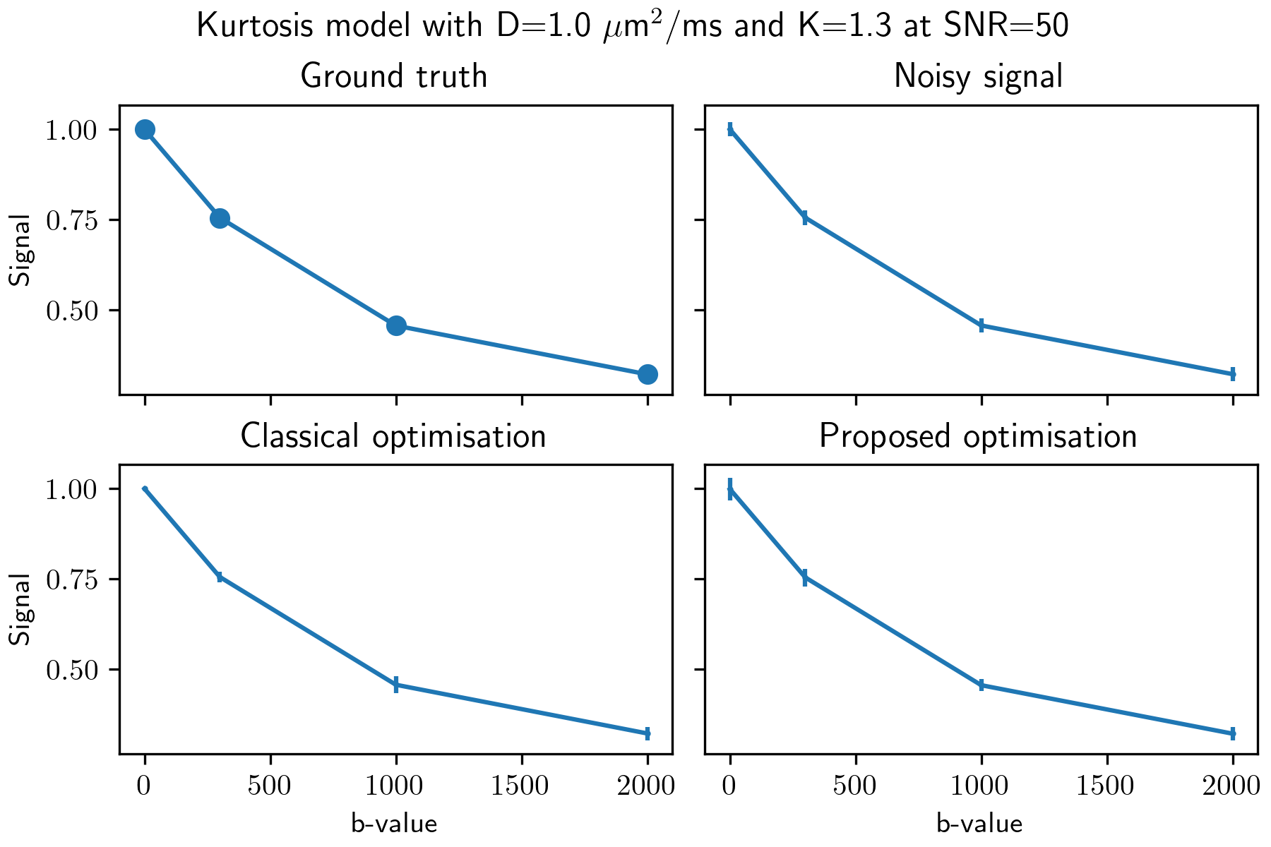
Figure 1: An example for 1000 realisations of a synthetic signal at SNR 50 with Rician distributed noise, that is the noise standard deviation is set to 1/50. The mean of the noisy signal is shown with the standard deviation of each realisation as the error bars. Similar results are obtained for both optimisation methods, but the classical optimisation takes approximately 7 seconds to process all voxels while the proposed method only takes 0.4 seconds by using the best matching value of the distribution.
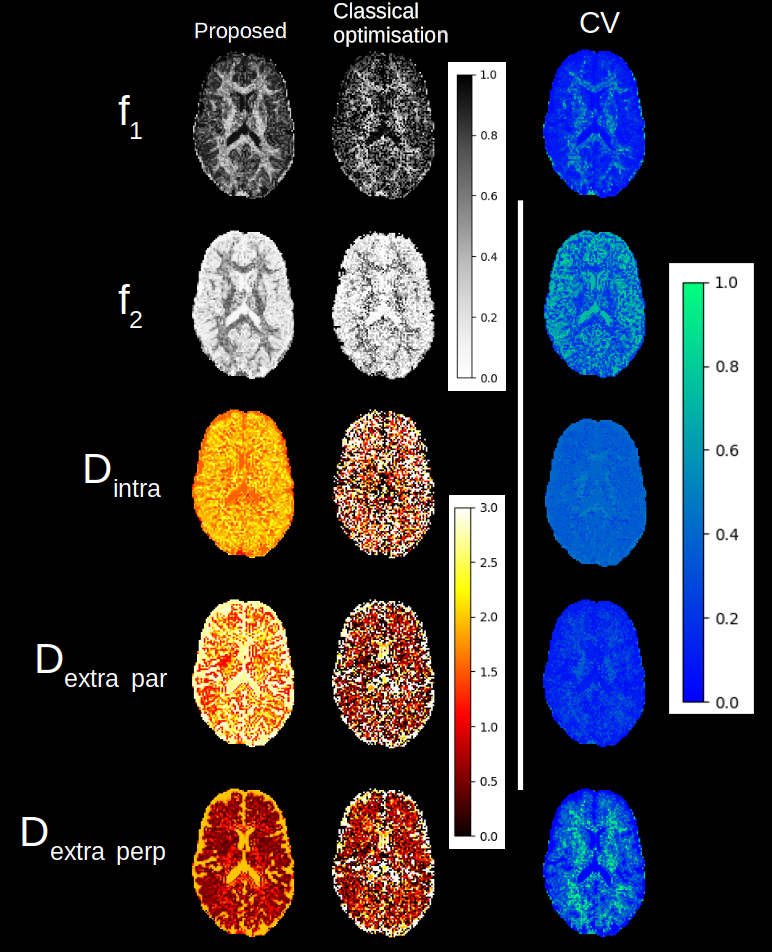
Figure 2: Parameters maps obtained with the proposed method and the classical optimisation for the stick and zeppelin model. On the right, variability of the parameters as computed from the coefficient of variation. Note the reduction in the number of white voxels for the diffusivities with the proposed method - a likely sign of degeneracy as the upper bound of 3 um2/ms is often achieved with the classical optimisation algorithm.
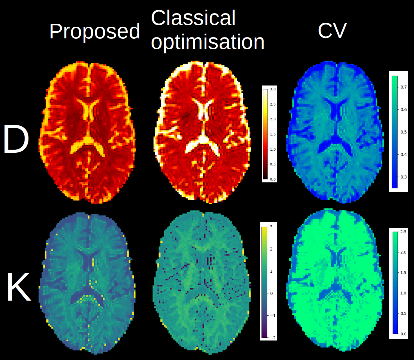
Figure 3: The computed mean diffusivity (top) and mean kurtosis (bottom) for the proposed and classical optimisation methods. Note the decrease in outliers and increased contrast on the kurtosis map obtained by ignoring implausible signals for the proposed method as they are discarded beforehand instead of using a constraint, which would complexify the optimisation problem in the process. On the right, the CV shows that a one parameter model might be inadequate as the value is higher in the white matter than in the gray matter or corticospinal fluid.
DOI: https://doi.org/10.58530/2023/5171