5167
Measurement of Extracellular Electrical Conductivity Using Conductivity Tensor Imaging
Bup Kyung Choi1, Nitish Katoch1, Ji Ae Park2, Tae Hoon Kim3, Young Hoe Hur4, Jin Woong Kim5, and Hyung Joong Kim1
1Department of Biomedical Engineering, Kyung Hee University, Seoul, Korea, Republic of, 2Division of Applied RI, Korea Institute of Radiological and Medical Science, Seoul, Korea, Republic of, 3Medical Convergence Research Center, Wonkwang University Hospital, Iksan, Korea, Republic of, 4Department of Hepato-Biliary-Pancreas Surgery, Chonnam National University Medical School, Gwangju, Korea, Republic of, 5Department of Radiology, Chosun University Hospital and Chosun University College of Medicine, Gwangju, Korea, Republic of
1Department of Biomedical Engineering, Kyung Hee University, Seoul, Korea, Republic of, 2Division of Applied RI, Korea Institute of Radiological and Medical Science, Seoul, Korea, Republic of, 3Medical Convergence Research Center, Wonkwang University Hospital, Iksan, Korea, Republic of, 4Department of Hepato-Biliary-Pancreas Surgery, Chonnam National University Medical School, Gwangju, Korea, Republic of, 5Department of Radiology, Chosun University Hospital and Chosun University College of Medicine, Gwangju, Korea, Republic of
Synopsis
Keywords: Electromagnetic Tissue Properties, Electromagnetic Tissue Properties, Electrical Conductivity, Low-frequency conductivity, High-field MRI, Tissue properties, Cell density imaging
Conductivity measured at low-frequency can provide information on extracellular space (ECS), which will be useful in clinical applications such as tumor imaging and bioelectromagnetic modeling. Recently proposed conductivity tensor imaging (CTI) technique provides the anisotropic low-frequency conductivity distribution extracted from high-frequency conductivity measurement from the B1 map of MRI. The extracellular conductivity measured using CTI from three phantoms was compared with an impedance analyzer. The accuracy of the CTI technique was estimated to be high enough for most clinical applications.Abstract
Changes in cellular structure, such as cell density and anisotropy, are detectable only at low-frequency because thin cell membranes are transparent at higher frequencies1,2. In this study, we aim to verify the contrast mechanism of the conductivity tensor imaging (CTI) technique using three conductivity phantoms made of cell-like material. The relative errors in the reconstructed CTI images with respect to the measured conductivity values using an impedance analyzer were in the range of 1.1 to 11.48%.Methods
We constructed three conductivity phantoms from acrylic material with an inner diameter of 40 mm, including a cell-alike material called giant vesicles3. Giant vesicles dispersed in an electrolyte were prepared as described by Moscho et al3. To check the separation of intracellular and extracellular space, we stained the giant vesicle with trypan blue 0.4% (Thermo Fisher Scientific. USA).Phantom #1 consists of three compartments, as shown in Fig. 1a. Electrolyte #1 (blue) and electrolyte #2 (gray) had different ion concentrations. Electrolyte #1 was a NaCl solution of 7.5 g/L, and electrolyte #2 was a solution with 3.5 g/L NaCl and 1 g/L CuSO4. The giant vesicle suspension (GVS) is shown in fig. 1a was filled with electrolyte #1 and suspended in the same electrolyte #1. Fig. 1b shows phantom #2 and has the same design as phantom #1. Phantom #2 contained three compartments: electrolytes #1 (yellow), #2 (blue), and giant vesicle suspension (yellow and blue). Hyaluronic acid and polyethylene glycol solution were added to electrolyte #1 to increase its viscosity. We added 3 g/L of NaCl, 10 g/L of polyethylene glycol , and 2 g/L of hyaluronic acid (Sigma-Aldrich, USA) to electrolyte #1. For electrolyte #2, it contained just 3 g/L of NaCl. In phantom #2, the giant vesicles were filled with electrolyte #2 and surrounded with electrolyte #1.
We constructed phantom #3 with four compartments: electrolyte, giant vesicle suspension #1, #2, #3. Target extracellular volume fractions of electrolyte and giant vesicle suspensions were 0.2, 0.4, 0.6, and 1. The electrolyte was a NaCl solution of 8 g/L, and the giant vesicle suspensions were filled with the electrolyte and suspended in the same electrolyte. These phantoms are built in a setting where phantom #1 is ion concentration controlled, phantom #2 is mobility controlled, and phantom #3 has cell density in control, respectively.
CTI experiments were performed in a 9.4 T research MRI scanner (Agilent Technologies, USA). The multi-echo spin-echo (MSE) imaging sequence was used to acquire B1 phase maps to reconstruct high-frequency conductivity images of the phantoms2. The single-shot spin-echo echo-planar (SS-SE-EPI) imaging sequence was used for multi-b-diffusion-weighted imaging. TR=1500 ms and TE =15, 30, 45, 60, 75 ms, FOV=60×60 mm2, slice thickness (0.5 mm), matrix size (128×128) were decided to make iso-voxel imaging (0.5 mm). The b-values (0, 50, 150, 300, 500, 700, 1000, 1400, 1800, 2200, 2600, 3000, 3500) of diffusion imaging were chosen based on the diffusion signal of phantoms2.
Results and Discussion
Fig. 1(b) shows the images of CTI parameter. Electrolyte #1 and giant vesicle suspension had a higher contrast than electrolyte #2 in high-frequency conductivity (σH) images because the concentration of ions was higher than that of electrolyte #2. As we used similar electrolyte #1 in giant vesicles, in σH, no contrast difference was observed, whereas σL* was lower. The measured value of extracellular conductivity in GVS #1 was 0.78 S/m, whereas the relative error compared to the impedance analyzer was 1.7 %. In phantom #2, the conductivity values were controlled by changing the mobility of electrolytes outside giant vesicles. The value of σL* was impacted by a change in extracellular diffusion coefficient (diso**) due to a change in mobility, and the observed relative error in GVS #2 was 2.13%. We also compared the conductivity value of electrolytes in both phantoms to impedance analyzer and found that the error ranges from 1.1 to 9.2 % in CTI method. In phantom #3, the values of extracellular volume fraction (α) measured ranged from 0.18 to 63, which corroborated well with the visual setting of cell density settings in phantom. Compared to impedance analyzer, the measured error ranges from 2.76 to 5.25 %. At higher frequencies, no contrast difference was observed in GVS #1 to #3 in phantom #3, as conductivity at higher frequency does not affect by cell density. Fig. 2a shows the Bland-Altman plot to confirm the agreement between CTI and impedance analyzer from three phantoms. Bias (mean difference) was -0.013 S/m, and the limits of agreement were -0.013 ± 0.039 S/m. Two methods agreed well since the bias values are close to 0 and all data were in between limits of agreement. 95% confidence intervals for the bias, upper, and lower limits of agreement were -0.013 ± 0.009, 0.066 ± 0.016 and -0.092 ± 0.016 S/m. Fig. 3 shows the table of CTI parameters values and relative error in all three phantoms.Conclusion
We applied electrodeless CTI method to image three conductivity phantoms including five electrolytes and giant vesicle suspensions. The effects of cell density, ion concentration, and mobility on the electrical conductivity could be clearly observed from reconstructed conductivity tensor images.Acknowledgements
This research was funded by the National Research Foundation of Korea (NRF) grants funded by the Korea government (No. 2019R1A2C2088573, 2020R1I1A3065215, 2020R1A2C200790611, 2021R1I1A3050277, 2020R1I1A1A01073871, 2021R1A2C2004299, 2022R1I1A1A01065565).References
1. S. Z. K. Sajib et al. Electrodeless conductivity tensor imaging (CTI) using MRI: Basic theory and animal experiments. Biomed. Eng. Lett. 2018;8:273–282.
2. Katoch N. “Conductivity tensor imaging of in-vivo human brain and experimental validation using giant vesicle suspension”. IEEE TMI 38, 1569-1577 (2019).
3. A. Moscho et al. Rapid preparation of giant unilamellar vesicles. Proc. Nat. Acad. Sci. 1996; 93:11443–11447.
Figures
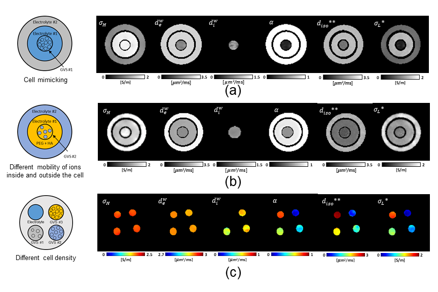
Fig. 1: Schematic illustration and images of CTI parameters for three conductivity phantoms (Phantom #1 to #3) with giant vesicles suspensions, where (σH) high-frequency conductivity, extracellular volume fraction (α), extracellular water diffusion coefficient (dew), intracellular water diffusion coefficient (diw), extracellular isotropic water diffusion coefficient (diso**), and low-frequency conductivity (σL*).
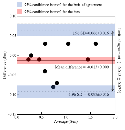
Fig. 2: Bland-Altman
plot of giant vesicle phantom #1, #2, and #3, where we compared the
conductivity values measured from CTI method to impedance analyzer.
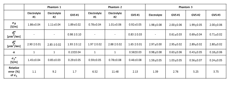
Table 1. Mean and standard deviation of CTI parameter and calculated relative error from impedance analyzer in low-frequency conductivity.
DOI: https://doi.org/10.58530/2023/5167