5026
Deep learning-based APT imaging using synthetically generated training data
Malvika Viswanathan1, Leqi Yin2, Yashwant Kurmi1, and Zhongliang Zu3
1Vanderbilt University Medical Center, Vanderbilt University Institute of Imaging Sciences, Nashville, TN, United States, 2Vanderbilt University, Nashville, TN, United States, 3Department of Radiology and Radiological Sciences, Vanderbilt University Institute of Imaging Sciences, Nashville, TN, United States
1Vanderbilt University Medical Center, Vanderbilt University Institute of Imaging Sciences, Nashville, TN, United States, 2Vanderbilt University, Nashville, TN, United States, 3Department of Radiology and Radiological Sciences, Vanderbilt University Institute of Imaging Sciences, Nashville, TN, United States
Synopsis
Keywords: Machine Learning/Artificial Intelligence, CEST & MT
Machine learning is increasingly applied to address challenges in specifically quantifying APT effect. The models are usually trained on measured data, which, however are usually lack of ground truth and sufficient training data. Synthetically generated data from both measurements and simulations can create training data which mimic tissues better than full simulations, cover all possible variations in sample parameters, and provide the ground truth. We evaluated the feasibility to use synthetic data to train models for predicting APT effect. Results show that the machine learning predicted APT is more close to the ground truth than the conventional multiple-pool Lorentzian fit.PURPOSE:
Amide proton transfer (APT) is a widely used application of chemical exchange saturation transfer (CEST) imaging for detecting mobile proteins/peptides and pH. APT-weighted imaging has been applied to diagnosing tumors, ischemic stroke, and multiple neurological diseases. Accurate APT imaging is critical for improving its applications. But this is still challenging till now. Multiple-pool Lorentzian fit has been used to isolate APT from confounding signals. However, its accuracy strongly depends on the imaging SNR, initial values, and boundaries. Recently, machine learning is increasingly applied to quantify CEST effects, which have shown better performance than the multiple-pool Lorentzian fit 1. Typically, the neural network is trained on measured data. However, the training using measured data usually have two limitations: 1) lack of ground truth data; 2) insufficient training data covering all possible variations in sample parameters. Synthetic data is an increasingly useful tool for training machine learning models when actual data is difficult to be obtained2. In this work, the model was trained with synthetically generated data from both measurements and simulations which mimic the tissues better than full simulations, cover all possible variations in most sample parameter, and provide the ground truth.METHODS:
Synthetic data were generated by$$ S(Δω)/S_0 =cos^2Ɵ R_{1w}/(R_{eff} (Δω)+R_{ex}^{APT} (Δω)+R_{ex}^{NOE} (Δω)+k_{amines} R_{ex}^{amines} (Δω)+k_{MT}R_{ex}^{MT} (Δω)) $$ (1)
In which S is the CEST signals with an RF frequency offset (Δω); $$$S_0$$$ is the control signal; $$$R_{eff},R_{ex}^{APT},R_{ex}^{NOE} ,R_{ex}^{amines} $$$ and $$$R_{ex}^{MT} $$$ represent water relaxation, APT, nuclear overhauser enhancement (NOE), and magnetization transfer (MT) in the rotating frame. $$$k_{amines}$$$ and $$$k_{MT} $$$are two scaling factors.
$$R_{eff }(Δω)=R_{1w} cos^2Ɵ+R_{2w} sin^2Ɵ$$ (2)
$$cos^2Ɵ=Δω^2/ω_1^2+Δω^2 ;$$ $$sin^2Ɵ=ω_1^2/ω_1^2+Δω^2$$
$$R_{ex}^{APT,NOE} (Δω)= f_{s} k_{sw} ω_1^2/(ω_1^2+(R_{2s}+k_{sw} ) k_{sw}+(Δω-Δ)^2 k_{sw}/(R_{2s}+k_{sw}))$$(3)
In which ω1 is the RF saturation power; fs and ksw are the solute concentration and solute-water exchange rate; Δ is the solute resonance frequency; R1w and R2w are the water longitudinal and transverse relaxation rates. R2s is the solute transverse relaxation rate. $$$R_{eff}$$$,$$$R_{ex}^{APT}$$$ and $$$R_{ex}^{NOE}$$$ were obtained from calculations of Eq. (2) and Eq. (3) with varied R1w, R2w, fs, and ksw. $$$R_{ex}^{amines}$$$ and $$$R_{ex}^{MT} $$$ were obtained from a multiple-pool (amide, amine, water, NOE, MT) Lorentzian fit of the average of the measured Z-spectra from normal tissues in rat brains. $$$ k_{amines}$$$ and $$$k_{MT}$$$ were varied to mimic the changes in amine CEST and MT effects. The input data consisted of the simulated raw Z-spectra from Eq. (1) with ω1 of 1µT, Δω from -10ppm to -5ppm, -0.5ppm to 0.5ppm, and 2.5ppm to 10ppm at 9.4T, and the corresponding R1w. The output data consisted of the amplitude (A) and width (W) of the amide pool which were calculated by 3.
$$A=f_{s} k_{sw} ω_1^2/(ω_1^2+(R_{2s}+k_{sw} ) k_{sw} ) $$
$$W=2\sqrt{ω_1^2 k_{sw}/(R_{2s}+k_{sw} )+k_{sw}^2 }$$ (4)
Total 3645 samples were generated, in which 90% were used for training and 10% were used for testing. A model with dense layers and a model with convolution layers were used to predict the A and W, respectively, which give better prediction than a single model. The machine learning predicted APT spectrum was obtained by calculating a Lorentzian function with the predicted A and W. The ground truth spectrum was obtained from Eq. (3). An overview of the data processing pipeline is given in Fig. 1. The difference between the machine learning predicted and the ground truth APT spectrum as well as the difference between the multiple-pool Lorentzian fitted and the ground truth APT spectrum (loss) from the test data were compared. The trained model was then applied to quantify the APT effect from the measured CEST Z-spectra on six rat brains bearing 9L tumors at 9.4T Varian MRI.
RESULTS:
Fig. 2 shows a representative input CEST Z-spectrum and the APT spectrum obtained from the machine learning prediction, multiple-pool Lorentzian fit, and the ground truth data. Note that the machine learning predicted APT spectrum is more close to the ground truth than that from the multiple-pool Lorentzian fit. Fig. 3 compares the loss of the machine learning method and the multiple-pool Lorentzian fit for all test data, which suggests that the machine learning method predicts the APT effect better than the multiple-pool Lorentzian fit. Fig. 4 shows measured CEST Z-spectra and the APT spectra from tumors and contralateral normal tissues. Fig. 5 shows maps of T2w-weighted, R1w, APT from machine learning prediction, and APT from the multiple-pool Lorentzian fit from a representative rat brain. There are nearly no contrast between tumor and contralateral normal tissue in Fig 5, which is in agreement with a previous report4.DISCUSSION AND CONCLUSION:
In diseases such as tumor, there are always changes in multiple sample parameters. The variations of these sample parameters in diseases with different types or stages are in a broad range. Training data from measurements on limited sample size may not cover all these changes. Using the inadequate amount of training data, the model may be overfitted and may not generalize well. In this work, we show the feasibility to use synthetically generated training data to train a model for predicting APT. We found that machine learning can provide better quantification of APT than the conventional multiple-pool Lorentzian fit.Acknowledgements
No acknowledgement found.References
- Glang F, Deshmane A, Prokudin S, Martin F, Herz K, Lindig T, et al. Deepcest 3t: Robust mri parameter determination and uncertainty quantification with neural networks-application to cest imaging of the human brain at 3t. Magnetic Resonance In Medicine. 2020;84:450-466
- Moya-Saez E, Pena-Nogales O, De Luis-Garcia R, Alberola-Lopez C. A deep learning approach for synthetic mri based on two routine sequences and training with synthetic data. Comput Meth Prog Bio. 2021;210
- Zaiss M, Schmitt B, Bachert P. Quantitative separation of cest effect from magnetization transfer and spillover effects by lorentzian-line-fit analysis of z-spectra. J Magn Reson. 2011;211:149-155
- Xu JZ, Zaiss M, Zu ZL, Li H, Xie JP, Gochberg DF, et al. On the origins of chemical exchange saturation transfer ( cest) contrast in tumors at 9.4 t. NMR in biomedicine. 2014;27:406-416
Figures
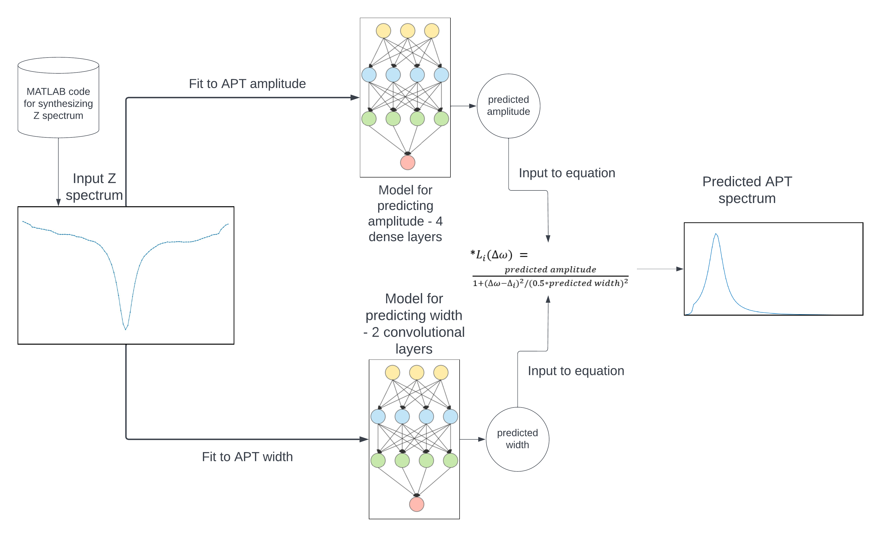
Figure1: Flowchart of machine learning method.
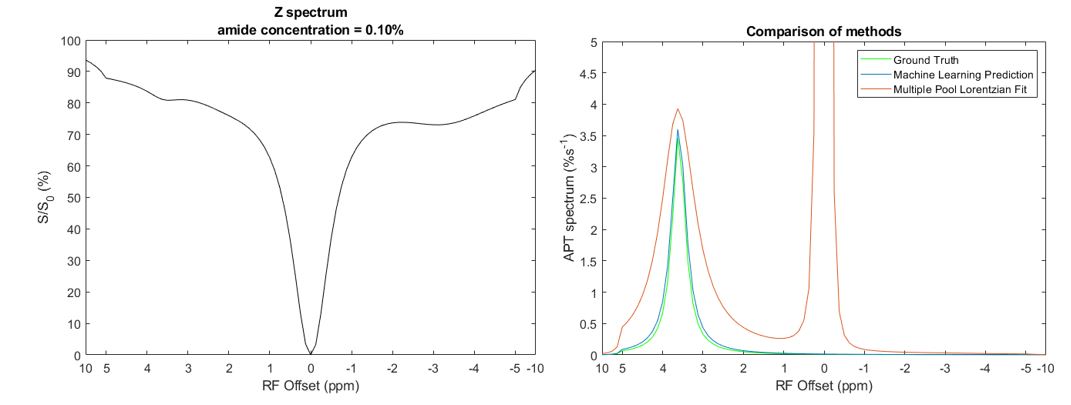
Figure2: CEST Z-spectrum and the APT
spectrum obtained with the machine prediction, multiple-pool Lorentzian fit,
and the ground truth data from a representative simulated sample for testing.
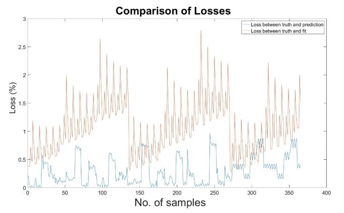
Figure3: Comparison
of the loss of the machine learning method and the multiple-pool Lorentzian fit
for all test data.
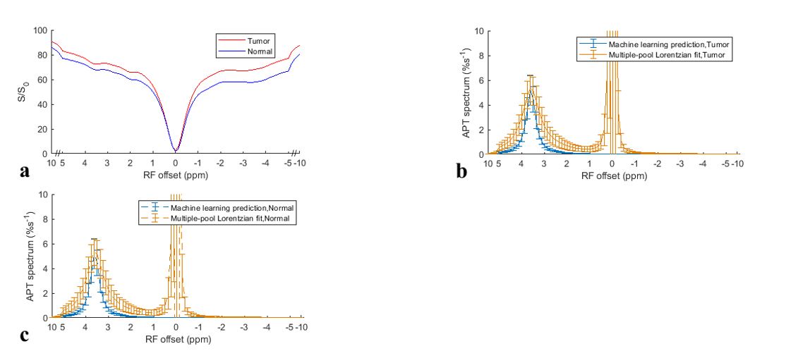
Figure4: Measured CEST
Z-spectra (a), APT spectrum from the machine learning prediction and the
multiple-pool Lorentzian fit from tumors (b) and from contralateral normal
tissues (c) of six rat brains.
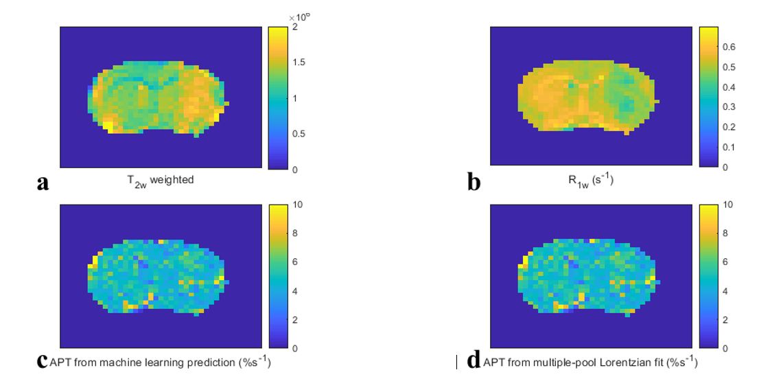
Figure5: Maps of T2w-weigthed (a), R1w (b),
APT from the machine learning prediction (c), and APT from the multiple-pool
Lorentzian fit (d) from a representative rat brain.
DOI: https://doi.org/10.58530/2023/5026