5017
Multiexponential analysis of diffusion exchange times reveals a distinct exchange process associated with metabolic activity
Teddy Xuke Cai1,2, Nathan Hu Williamson1, Rea Ravin1,3, and Peter Joel Basser1
1Eunice Kennedy Shriver National Institute of Child Health and Human Development, National Institutes of Health, Bethesda, MD, United States, 2Wellcome Centre for Integrative Neuroimaging, FMRIB, Nuffield Department of Clinical Neurosciences, University of Oxford, Oxford, United Kingdom, 3Celoptics, Inc., Rockville, MD, United States
1Eunice Kennedy Shriver National Institute of Child Health and Human Development, National Institutes of Health, Bethesda, MD, United States, 2Wellcome Centre for Integrative Neuroimaging, FMRIB, Nuffield Department of Clinical Neurosciences, University of Oxford, Oxford, United Kingdom, 3Celoptics, Inc., Rockville, MD, United States
Synopsis
Keywords: Diffusion/other diffusion imaging techniques, Data Analysis, Exchange
Contrary to prevailing views, recent work suggests that steady-state water exchange between the intra- and extracellular space is driven, in part, by active metabolic processes. To support these findings, we investigate whether exchange exhibits multiexponential behavior consistent with distinct exchange processes. We find a bimodal distribution of exchange times in live neural tissue, with only the faster peak being reduced upon the introduction of a sodium-potassium pump inhibitor, thus supporting the existence of active exchange. Furthermore, we describe a time-efficient method of isolating exchange and fitting multiexponential exchange times using diffusion exchange spectroscopy, paving the way for future studies.Introduction
The exchange of water between biological microenvironments, namely between the intra- and extracellular space, is generally considered to be a passive process mediated by membrane permeability. Recent work, however, suggests that exchange (as measured by diffusion MR) is linked to active, i.e., ATP-driven metabolic processes. Specifically, the exchange rate, $$$k$$$, has been linked to the activity of the sodium-potassium pump.1,2 Quantifying $$$k$$$ may provide functional information at the cellular level, representing, potentially, a non-BOLD-based form of functional MR. While promising, questions remain concerning both the methodology of measuring $$$k$$$ and its underlying biological correlates.Here we explore whether exchange is adequately described by a single parameter. Indeed, the existence of active exchange would imply, at the least, two distinct exchange processes – the passive permeability of the cell membrane, and exchange coupled to active processes like ion transport – for which there is no a priori reason to assume equal rates. Moreover, $$$k$$$ should scale with the local surface-to-volume ratio.3,4 Therefore, we hypothesize that exchange times are broadly distributed with potentially well-separated active and passive peaks.
To test this hypothesis, we measure probability distribution functions of the exchange time, $$$P(\tau_k)=P(1/k)$$$, by applying multiexponential analysis using numerical inverse Laplace transforms (ILTs) to data in which the effect of exchange has been isolated. Using a low-field, static gradient system, $$$P(\tau_k)$$$ data were acquired from ex vivo neonatal mouse spinal cords in three conditions: fixed, live, and live whilst treated with ouabain, a sodium-potassium pump inhibitor.
Theory
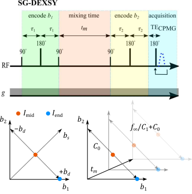
Previously, we demonstrated that the diffusion exchange spectroscopy5 (DEXSY) sequence, in which two parallel diffusion encodings with b-values $$$b_1$$$ and $$$b_2$$$ are separated by a mixing time, $$$t_m$$$, can be leveraged to measure exchange whilst heavily sub-sampling the $$$(b_1,b_2)$$$ domain.6-8 First, the signal variation is measured along an axis of constant total diffusion weighting $$$b_s=b_1+b_2$$$, removing the effects of non-exchanging, Gaussian diffusion. Next, taking a ratio of signals at each $$$t_m$$$ normalizes $$$T_1$$$ relaxation. Finally, by varying $$$t_m$$$, the effect of exchange (during $$$t_m$$$) is isolated.The apparent exchanging signal fraction $$$f_{\mathrm{exch}}(t_m)$$$ is proportional to a log-ratio of the signal $$$I(b_1,b_2,t_m)$$$ at the midpoint $$$I_{\mathrm{mid}}(t_m)=I(\tfrac{b_s}{2},\tfrac{b_s}{2},t_m)$$$ and endpoint $$$I_{\mathrm{end}}(t_m)=I(b_s,0,t_m)$$$ of the $$$b_d=b_1-b_2$$$ axis, normalizing to $$$t_m=0$$$ (Fig. 1):
$$f_{\mathrm{exch}}(t_m)=C_1\left[\ln\left(\frac{I_{\mathrm{mid}}(t_m)}{I_{\mathrm{end}}(t_m)}\right)-C_0\right],\;\;C_0=\ln\left(\frac{I_{\mathrm{mid}}(0)}{I_{\mathrm{end}}(0)}\right),$$
where $$$C_1$$$ is a proportionality constant. Note that $$$C_0$$$ encompasses restriction, exchange during encodings, and other effects invariant with $$$t_m$$$.8 Exchange is modelled as
$$f_{\mathrm{exch}}(t_m)=f_\infty\left[1-\int_0^\infty\exp\left(-\frac{t_m}{\tau_k}\right)P(\tau_k)d\tau_k\right],$$
where $$$f_\infty=\lim_{t_m\to\infty}f_{\mathrm{exch}}(t_m)$$$ is the steady-state exchange fraction, corresponding to complete volume turnover between compartments. Rearranging and substituting Eq. (1), $$$C_1$$$ cancels and
$$1-\frac{f_{\mathrm{exch}}(t_m)}{f_\infty}=1-\left[\frac{\ln\left(\frac{I_{\mathrm{mid}}(t_m)}{I_{\mathrm{end}}(t_m)}\right)-C_0}{\lim_{t_m\to\infty}\ln\left(\frac{I_{\mathrm{mid}}(t_m)}{I_{\mathrm{end}}(t_m)}\right)-C_0}\right]=\int_0^\infty\exp\left(-\frac{t_m}{\tau_k}\right)P(\tau_k)d\tau_k,$$
which is amenable to using an ILT to obtain $$$P(\tau_k)$$$.
Methods
The static gradient DEXSY (SG-DEXSY) pulse sequence (Fig. 1) was implemented on a PM-10 NMR MOUSE9 single-sided magnet at $$$\omega_0=13.79\;\mathrm{MHz}$$$, $$$B_0=0.3239\;\mathrm{T}$$$, $$$g=15.3\;\mathrm{T/m}$$$ with a home-built solenoid RF coil and test chamber.10 RF pulse lengths $$$=2/2\;\mu\mathrm{s}$$$, pulse powers $$$=-22/-16\;\mathrm{dB}$$$, $$$\mathrm{TR}=2\;\mathrm{s}$$$, 8000 echo CPMG train with $$$\mathrm{TE}=25\;\mu\mathrm{s}$$$, 8 points per echo, and $$$0.5\;\mu\mathrm{s}$$$ dwell time.Live (i.e., viable) and fixed ex vivo neonatal (postnatal day 1–4) mouse spinal cords were studied. Spinal cords were bathed in artificial cerebrospinal fluid at 95% O2/5% CO2 and $$$25^{\circ}\mathrm{C}$$$. For the ouabain treatment condition, ouabain was added at a saturating concentration of $$$100\;\mu\mathrm{M}$$$.1
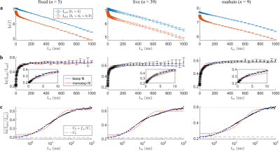
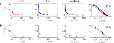
Data were acquired at $$$b_s=4.5\;\mathrm{ms}/\mu\mathrm{m}^2$$$ over 69 values of $$$t_m=0.2-1000\;\mathrm{ms}$$$. A biexponential fit to the log-ratio of signals was first performed to yield robust estimates of the intercept $$$C_0$$$ and limit $$$f_\infty/C_1$$$ (Figs. 2a–c). The data were then renormalized following Eq. (3) (Fig. 3) before performing an ILT using the Butler-Reeds-Dawson algorithm11,12 with 200 points spaced log-linearly from $$$\tau_k=1\times10^{-3}-1\times10^{-4}\;\mathrm{ms}$$$. Data were also sub-sampled to 15 values of $$$t_m$$$ (Fig. 3b) to assess the stability of the inversion with minimal data, inverting with 50 points from $$$\tau_k=1\times10^{-2}-1\times10^{3}\;\mathrm{ms}$$$.
Results
Inverted $$$P(\tau_k)$$$ distributions from fully sampled (Fig. 4a) and sub-sampled (Fig. 4b) data are presented for the live, fixed, and live with ouabain conditions. The distributions are scaled by $$$f_\infty/C_1$$$ to facilitate comparison in absolute terms. The distributions are broad. Live tissue exhibits a bimodal distribution with peaks centered at 2 and 72 $$$\mathrm{ms}$$$. In the ouabain case, the faster peak is reduced. Fixed tissue is approximately unimodal. The sub-sampled case shows similar trends, albeit less resolved. Importantly, the distinct, short $$$\tau_k$$$ peak in live tissue remains.Discussion
Our results support that active and passive exchange have well-separated exchange times. Of the two peaks in live tissue, only the faster peak is reduced with ouabain, suggesting that fast exchange, specifically, is an active process. Furthermore, we find that $$$P(\tau_k)$$$ is broadly distributed, consistent with a dependence on local microstructure. Pairing $$$P(\tau_k)$$$ estimation with other modalities, namely diffusion modelling, may provide additional information about inter-compartment exchange.Our method is uniquely suited to such analysis. Other time-efficient methods of measuring exchange (e.g., FEXSY13, the Kärger model14, etc.), generally rely on multi-parametric fitting of the signal as exchange is not isolated. This greatly complicates the application of ILTs to study exchange. In contrast, the presented approach reduces to a form in which the signal is dependent only on exchange. Remaining parameters ($$$C_0,f_\infty/C_1$$$) are experimentally observable (Fig. 2c) leaving a simple kernel. Thus, we believe that our method is optimal for such analysis.
Acknowledgements
The authors would like to thank Dr. Melanie Falgairolle and Dr. Michael James O'Donovan for assistance with the preparation of spinal cords and the protocol for ouabain perturbation.References
- N. H. Williamson et al., “Water exchange rates measure active transport and homeostasis in neural tissue”, bioRxiv, 2022. doi: 10.1101/2022.09.23.483116
- C. S. Springer et al. “Metabolic activity diffusion imaging (MADI): II. Noninvasive, high-resolution human brain mapping of sodium pump flux and cell metrics”, NMR in Biomedicine, e4782, 2022.
- D. S. Novikov, E. Fieremans, J. H. Jensen, and J. A. Helpern, “Random walks with barriers”, Nature Physics, vol. 7, pp. 508–514, 2011.
- C. S. Springer. et al. “Metabolic activity diffusion imaging (MADI): I. Metabolic, cytometric modeling and simulations”, NMR in Biomedicine, e4781, 2022.
- P. T. Callaghan and I. Furó, “Diffusion-diffusion correlation and exchange as a signature for local order and dynamics”, Journal of Chemical Physics, vol. 120, no. 8, pp. 4032-4038, 2004.
- T. X. Cai, D. Benjamini, M. E. Komlosh, P. J. Basser, and N. H. Williamson, "Rapid detection of the presence of diffusion exchange," Journal of Magnetic Resonance, vol. 297, pp. 17-22, 2018.
- N. H. Williamson et al., "Real-time measurement of diffusion exchange rate in biological tissue," Journal of Magnetic Resonance, vol. 317, 106782, 2020.
- T. X. Cai, N. H. Williamson, R. Ravin, and P. J. Basser, "Disentangling the effects of restriction and exchange with diffusion exchange spectroscopy," Frontiers in Physics, 805793, 2022.
- G. Eidmann, R. Savelsberg, P. Blümler, and B. Blümich, "The NMR MOUSE, a mobile universal surface explorer," Journal of Magnetic Resonance, Series A, vol. 122, no. 1, pp. 104-109, 1996.
- N. H. Williamson et al., "Magnetic resonance measurements of cellular and sub-cellular membrane structures in live and fixed neural tissue," eLife, vol. 8, e51101, 2019.
- Ohkubo, T. “Open source 1d/2d inverse laplace program,” 2022. Available at: https://amorphous.tf.chiba-u.jp/memo.files/osilap/osilap.html (Accessed: October 24, 2022).
- J. P. Butler, J. A. Reeds, and S. V. Dawson, “Estimating Solutions of First Kind Integral Equations with Nonnegative Constraints and Optimal Smoothing”, SIAM Journal on Numerical Analysis, vol. 18, no. 3, pp. 381–397, 1981.
- I. Åslund, A. Nowacka, M. Nilsson, and D. Topgaard, “Filter-exchange PGSE NMR determination of cell membrane permeability”, Journal of Magnetic Resonance, vol. 200, no. 2, pp. 291–295, 2009.
- Kärger J, “NMR self-diffusion studies in heterogeneous systems”, Advances in Colloid and Interface Science, vol. 23, pp. 129–148, 1985.
Figures

Figure 1: Pulse sequence and $$$(b_1,b_2)$$$ sampling scheme. Static gradient DEXSY (SG-DEXSY) pulse sequence implemented on a PM-10 NMR MOUSE single-sided system. Signal is summed in a CPMG echo train to maximize SNR. Signal is measured at $$$I_\mathrm{mid}\;(b_1=b_2=b_s/2)$$$ and $$$I_\mathrm{end}\;(b_1=b_s)$$$ at various $$$t_m$$$. The log-ratio of $$$I_\mathrm{mid}$$$ and $$$I_\mathrm{end}$$$ is proportional to $$$f_\mathrm{exch}(t_m)$$$ by $$$C_1$$$, less the intercept at $$$t_m=0$$$, $$$C_0$$$. At long $$$t_m$$$, the limit $$$f_\infty/C_1$$$ is reached.

Figure 2: Data processing and fitting for $$$C_0,f_\infty/C_1$$$. (a) Raw data from summed CPMG echoes at $$$I_\mathrm{mid}$$$ and $$$I_\mathrm{end}$$$. Error bars = ±1 SD from repeated measurements on a sample. (b) Log-ratio of the signals with biexponential and monoexponential fits. (c) Same as (b) but with a log $$$t_m$$$ axis and showing only mean values. Here, $$$f_\infty/C_1$$$ and $$$C_0$$$ are visible as bounds well-fit with a biexponential. Fitted values are $$$f_\infty/C_1=[0.331,0.418,0.369]$$$ and $$$C_0=[0.198,0.213,0.220]$$$, left to right.

Figure 3: Data renormalized into an exponential decay form. Using the previous biexponential fit in Fig. 2 and Eq. (3), data is transformed into a form that is invertible using an ILT. (a) Fully sampled data with 69 values of $$$t_m$$$, taking only the mean log-ratio signal values. On the right is a combined log $$$t_m$$$ plot. (b) Sub-sampled data over the same range at $$$t_m=[0.2,1,2,4,7,12,18,32,50,80,120,220,340,600,1000]\; \mathrm{ms}.$$$ Note that fits for $$$f_\infty/C_1$$$ and $$$C_0$$$ were performed again with the sub-sampled data.

Figure 4: Inverted $$$P(\tau_k)$$$ distributions in the fully sampled and sub-sampled cases for fixed, live, and live with ouabain spinal cords. (a) Distributions in the fully sampled case (Fig. 3a). Distributions are scaled by $$$f_\infty/C_1$$$ for comparison in terms of the total exchange during $$$t_m$$$. The center of the two peaks in live tissue are marked (2,79 ms). (b) $$$P(\tau_k)$$$ in the sub-sampled case (Fig. 3b). While less resolved, characteristics are broadly similar to (a), suggesting the feasibility of data reduction.
DOI: https://doi.org/10.58530/2023/5017